FantasyFootball marks prediction
In this second part of the analysis, we will apply some machine learning techniques to predict the performances of the football players.
#import

import pandas as pd
import numpy as np
import matplotlib.pyplot as plt
marks_final= pd.read_csv('dataset_2015_marks.csv', index_col=0)
from sklearn.feature_selection import SelectKBest
from sklearn.feature_selection import chi2
marks_final.rename(columns = {'LastMark':'lastMark'})
marks_final.head()
| player | name | team | day | goal | penalty | owngoal | mark | rankOwnTeam | playingHome | opponentTeam | rankOpponentTeam | avgPrevious5 | avgSoFar | LastMark | isSuff | |
|---|---|---|---|---|---|---|---|---|---|---|---|---|---|---|---|---|
| 0 | 2247 | Sportiello | Atalanta | 1 | 0 | 0 | 0 | 7.0 | 10 | 1 | Verona | 10 | NaN | NaN | NaN | 1 |
| 1 | 2247 | Sportiello | Atalanta | 2 | 0 | 0 | 0 | 7.5 | 10 | 0 | Cagliari | 10 | 7.000000 | 7.000000 | 7.0 | 1 |
| 2 | 2247 | Sportiello | Atalanta | 3 | 0 | 0 | 0 | 6.0 | 5 | 1 | Fiorentina | 15 | 7.250000 | 7.250000 | 7.5 | 1 |
| 3 | 2247 | Sportiello | Atalanta | 4 | 0 | 0 | 0 | 6.5 | 9 | 0 | Inter | 6 | 6.833333 | 6.833333 | 6.0 | 1 |
| 4 | 2247 | Sportiello | Atalanta | 5 | 0 | 0 | 0 | 5.0 | 11 | 1 | Juventus | 1 | 6.750000 | 6.750000 | 6.5 | 0 |
As a filling value for the statistics, let us put 5 at the moment. Not too bad but not good. Let’s say that in the doubt we are peximistic
marks_final = marks_final.fillna(5)
marks_final.head()
| player | name | team | day | goal | penalty | owngoal | mark | rankOwnTeam | playingHome | opponentTeam | rankOpponentTeam | avgPrevious5 | avgSoFar | LastMark | isSuff | |
|---|---|---|---|---|---|---|---|---|---|---|---|---|---|---|---|---|
| 0 | 2247 | Sportiello | Atalanta | 1 | 0 | 0 | 0 | 7.0 | 10 | 1 | Verona | 10 | 5.000000 | 5.000000 | 5.0 | 1 |
| 1 | 2247 | Sportiello | Atalanta | 2 | 0 | 0 | 0 | 7.5 | 10 | 0 | Cagliari | 10 | 7.000000 | 7.000000 | 7.0 | 1 |
| 2 | 2247 | Sportiello | Atalanta | 3 | 0 | 0 | 0 | 6.0 | 5 | 1 | Fiorentina | 15 | 7.250000 | 7.250000 | 7.5 | 1 |
| 3 | 2247 | Sportiello | Atalanta | 4 | 0 | 0 | 0 | 6.5 | 9 | 0 | Inter | 6 | 6.833333 | 6.833333 | 6.0 | 1 |
| 4 | 2247 | Sportiello | Atalanta | 5 | 0 | 0 | 0 | 5.0 | 11 | 1 | Juventus | 1 | 6.750000 | 6.750000 | 6.5 | 0 |
desc = marks_final.describe()
print(desc)
            player          day         goal      penalty      owngoal  \
count  9904.000000  9904.000000  9904.000000  9904.000000  9904.000000
mean   2468.801393    19.501817     0.091680     0.008380     0.003332
std     140.635213    10.996809     0.315661     0.093354     0.057630
min    2247.000000     1.000000     0.000000     0.000000     0.000000
25%    2351.000000    10.000000     0.000000     0.000000     0.000000
50%    2458.000000    20.000000     0.000000     0.000000     0.000000
75%    2572.000000    29.000000     0.000000     0.000000     0.000000
max    2820.000000    38.000000     3.000000     2.000000     1.000000

              mark  rankOwnTeam  playingHome  rankOpponentTeam  avgPrevious5  \
count  9904.000000  9904.000000  9904.000000       9904.000000   9904.000000
mean      5.913318    10.341882     0.498485         10.332593      5.859603
std       0.690952     5.673185     0.500023          5.664493      0.500290
min       3.000000     1.000000     0.000000          1.000000      4.000000
25%       5.500000     5.000000     0.000000          5.000000      5.500000
50%       6.000000    10.000000     0.000000         10.000000      5.900000
75%       6.500000    15.000000     1.000000         15.000000      6.200000
max       8.500000    20.000000     1.000000         20.000000      8.250000

          avgSoFar     LastMark       isSuff
count  9904.000000  9904.000000  9904.000000
mean      5.884887     5.722032     0.622779
std       0.389586     0.725208     0.484716
min       4.000000     4.000000     0.000000
25%       5.684211     5.000000     0.000000
50%       5.928571     5.500000     1.000000
75%       6.125000     6.000000     1.000000
max       8.000000     8.500000     1.000000
Ok now we should switch on our brain. In order to maximize the performance of our classifiers, we should:
- study the correlated features (a lot of them, especially the engineered ones)
- pay attention to the categorical features (even if we transform them into integers, we do not want that our algorithm think that they could be ordererd)
- some of the algorithms we want to try expects features centered in zero (we will surely try SVM since our predicted lable is binary)
from sklearn.preprocessing import LabelEncoder, OneHotEncoder
# Get one hot encoding of columns team
one_hot = pd.get_dummies(marks_final['team'])
marks_final = marks_final.join(one_hot)
marks_final.head()
| player | name | team | day | goal | penalty | owngoal | mark | rankOwnTeam | playingHome | ... | Milan | Napoli | Palermo | Parma | Roma | Sampdoria | Sassuolo | Torino | Udinese | Verona | |
|---|---|---|---|---|---|---|---|---|---|---|---|---|---|---|---|---|---|---|---|---|---|
| 0 | 2247 | Sportiello | Atalanta | 1 | 0 | 0 | 0 | 7.0 | 10 | 1 | ... | 0 | 0 | 0 | 0 | 0 | 0 | 0 | 0 | 0 | 0 |
| 1 | 2247 | Sportiello | Atalanta | 2 | 0 | 0 | 0 | 7.5 | 10 | 0 | ... | 0 | 0 | 0 | 0 | 0 | 0 | 0 | 0 | 0 | 0 |
| 2 | 2247 | Sportiello | Atalanta | 3 | 0 | 0 | 0 | 6.0 | 5 | 1 | ... | 0 | 0 | 0 | 0 | 0 | 0 | 0 | 0 | 0 | 0 |
| 3 | 2247 | Sportiello | Atalanta | 4 | 0 | 0 | 0 | 6.5 | 9 | 0 | ... | 0 | 0 | 0 | 0 | 0 | 0 | 0 | 0 | 0 | 0 |
| 4 | 2247 | Sportiello | Atalanta | 5 | 0 | 0 | 0 | 5.0 | 11 | 1 | ... | 0 | 0 | 0 | 0 | 0 | 0 | 0 | 0 | 0 | 0 |
5 rows × 36 columns
We should do the same with the opponent. If we do this, though, there could be some overlapping. so we have to rename the teams if we are talking about opponents
one_hot = pd.get_dummies(marks_final['opponentTeam'])
one_hot.head()
| Atalanta | Cagliari | Cesena | Chievo | Empoli | Fiorentina | Genoa | Inter | Juventus | Lazio | Milan | Napoli | Palermo | Parma | Roma | Sampdoria | Sassuolo | Torino | Udinese | Verona | |
|---|---|---|---|---|---|---|---|---|---|---|---|---|---|---|---|---|---|---|---|---|
| 0 | 0 | 0 | 0 | 0 | 0 | 0 | 0 | 0 | 0 | 0 | 0 | 0 | 0 | 0 | 0 | 0 | 0 | 0 | 0 | 1 |
| 1 | 0 | 1 | 0 | 0 | 0 | 0 | 0 | 0 | 0 | 0 | 0 | 0 | 0 | 0 | 0 | 0 | 0 | 0 | 0 | 0 |
| 2 | 0 | 0 | 0 | 0 | 0 | 1 | 0 | 0 | 0 | 0 | 0 | 0 | 0 | 0 | 0 | 0 | 0 | 0 | 0 | 0 |
| 3 | 0 | 0 | 0 | 0 | 0 | 0 | 0 | 1 | 0 | 0 | 0 | 0 | 0 | 0 | 0 | 0 | 0 | 0 | 0 | 0 |
| 4 | 0 | 0 | 0 | 0 | 0 | 0 | 0 | 0 | 1 | 0 | 0 | 0 | 0 | 0 | 0 | 0 | 0 | 0 | 0 | 0 |
one_hot.columns = "Opp:"+one_hot.columns
one_hot.head()
| Opp:Atalanta | Opp:Cagliari | Opp:Cesena | Opp:Chievo | Opp:Empoli | Opp:Fiorentina | Opp:Genoa | Opp:Inter | Opp:Juventus | Opp:Lazio | Opp:Milan | Opp:Napoli | Opp:Palermo | Opp:Parma | Opp:Roma | Opp:Sampdoria | Opp:Sassuolo | Opp:Torino | Opp:Udinese | Opp:Verona | |
|---|---|---|---|---|---|---|---|---|---|---|---|---|---|---|---|---|---|---|---|---|
| 0 | 0 | 0 | 0 | 0 | 0 | 0 | 0 | 0 | 0 | 0 | 0 | 0 | 0 | 0 | 0 | 0 | 0 | 0 | 0 | 1 |
| 1 | 0 | 1 | 0 | 0 | 0 | 0 | 0 | 0 | 0 | 0 | 0 | 0 | 0 | 0 | 0 | 0 | 0 | 0 | 0 | 0 |
| 2 | 0 | 0 | 0 | 0 | 0 | 1 | 0 | 0 | 0 | 0 | 0 | 0 | 0 | 0 | 0 | 0 | 0 | 0 | 0 | 0 |
| 3 | 0 | 0 | 0 | 0 | 0 | 0 | 0 | 1 | 0 | 0 | 0 | 0 | 0 | 0 | 0 | 0 | 0 | 0 | 0 | 0 |
| 4 | 0 | 0 | 0 | 0 | 0 | 0 | 0 | 0 | 1 | 0 | 0 | 0 | 0 | 0 | 0 | 0 | 0 | 0 | 0 | 0 |
marks_final = marks_final.join(one_hot)
marks_final.head()
| player | name | team | day | goal | penalty | owngoal | mark | rankOwnTeam | playingHome | ... | Opp:Milan | Opp:Napoli | Opp:Palermo | Opp:Parma | Opp:Roma | Opp:Sampdoria | Opp:Sassuolo | Opp:Torino | Opp:Udinese | Opp:Verona | |
|---|---|---|---|---|---|---|---|---|---|---|---|---|---|---|---|---|---|---|---|---|---|
| 0 | 2247 | Sportiello | Atalanta | 1 | 0 | 0 | 0 | 7.0 | 10 | 1 | ... | 0 | 0 | 0 | 0 | 0 | 0 | 0 | 0 | 0 | 1 |
| 1 | 2247 | Sportiello | Atalanta | 2 | 0 | 0 | 0 | 7.5 | 10 | 0 | ... | 0 | 0 | 0 | 0 | 0 | 0 | 0 | 0 | 0 | 0 |
| 2 | 2247 | Sportiello | Atalanta | 3 | 0 | 0 | 0 | 6.0 | 5 | 1 | ... | 0 | 0 | 0 | 0 | 0 | 0 | 0 | 0 | 0 | 0 |
| 3 | 2247 | Sportiello | Atalanta | 4 | 0 | 0 | 0 | 6.5 | 9 | 0 | ... | 0 | 0 | 0 | 0 | 0 | 0 | 0 | 0 | 0 | 0 |
| 4 | 2247 | Sportiello | Atalanta | 5 | 0 | 0 | 0 | 5.0 | 11 | 1 | ... | 0 | 0 | 0 | 0 | 0 | 0 | 0 | 0 | 0 | 0 |
5 rows × 56 columns
ok done! focus now on correlations
import seaborn as sns
marks_final.columns
Index([u'player', u'name', u'team', u'day', u'goal', u'penalty', u'owngoal',
       u'mark', u'rankOwnTeam', u'playingHome', u'opponentTeam',
       u'rankOpponentTeam', u'avgPrevious5', u'avgSoFar', u'LastMark',
       u'isSuff', u'Atalanta', u'Cagliari', u'Cesena', u'Chievo', u'Empoli',
       u'Fiorentina', u'Genoa', u'Inter', u'Juventus', u'Lazio', u'Milan',
       u'Napoli', u'Palermo', u'Parma', u'Roma', u'Sampdoria', u'Sassuolo',
       u'Torino', u'Udinese', u'Verona', u'Opp:Atalanta', u'Opp:Cagliari',
       u'Opp:Cesena', u'Opp:Chievo', u'Opp:Empoli', u'Opp:Fiorentina',
       u'Opp:Genoa', u'Opp:Inter', u'Opp:Juventus', u'Opp:Lazio', u'Opp:Milan',
       u'Opp:Napoli', u'Opp:Palermo', u'Opp:Parma', u'Opp:Roma',
       u'Opp:Sampdoria', u'Opp:Sassuolo', u'Opp:Torino', u'Opp:Udinese',
       u'Opp:Verona'],
      dtype='object')
marks_final.columns[:16]
Index([u'player', u'name', u'team', u'day', u'goal', u'penalty', u'owngoal',
       u'mark', u'rankOwnTeam', u'playingHome', u'opponentTeam',
       u'rankOpponentTeam', u'avgPrevious5', u'avgSoFar', u'LastMark',
       u'isSuff'],
      dtype='object')
marks_final.columns[:16].difference(['player','name','team','opponentTeam'])
Index([u'LastMark', u'avgPrevious5', u'avgSoFar', u'day', u'goal', u'isSuff',
       u'mark', u'owngoal', u'penalty', u'playingHome', u'rankOpponentTeam',
       u'rankOwnTeam'],
      dtype='object')
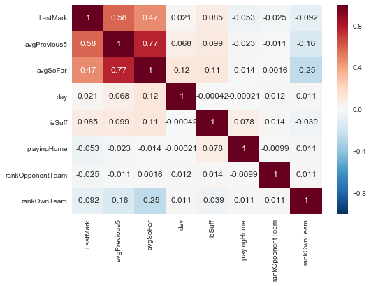
corr = marks_final[marks_final.columns[:16].difference(['player','name','team','opponentTeam','goal','owngoal','mark','penalty'])].corr()
_ = sns.heatmap(corr, annot = True)
plt.show()
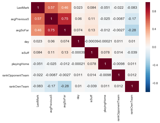
corr = marks_final[marks_final.columns[:16].difference(['player','name','team','opponentTeam','goal','owngoal','mark','penalty'])].corr(method='spearman')
sns.heatmap(corr, annot = True)
plt.show()
from scipy.stats import pointbiserialr
We have used spearman and pearson. We have seen that the only features strongly correlated are the averages, as predictable. let’s use biserial correlation for binary features
def correlation(X,Y):
    param = []
    correlation=[]
    abs_corr=[]
    columns = marks_final.columns[:16].difference(['player','name','team','opponentTeam','goal','owngoal','mark','penalty'])


    for c in columns:
        corr = pointbiserialr(X[c],Y)[0]
        correlation.append(corr)
        param.append(c)
        abs_corr.append(abs(corr))
    print correlation
    #create data frame
    param_cor = pd.DataFrame({'correlation':correlation,'parameter':param, 'abs_corr':abs_corr})
    paramc_cor=param_cor.sort_values(by=['abs_corr'], ascending=False)
    param_cor=param_cor.set_index('parameter')


    print param_cor
correlation(marks_final, marks_final['isSuff'])
[0.08503341229851559, 0.099145358562043442, 0.112238463187295, -0.00042075422779776981, 1.0, 0.078053212529890642, 0.013959624950329314, -0.039171776122582443]
                  abs_corr  correlation
parameter
LastMark          0.085033     0.085033
avgPrevious5      0.099145     0.099145
avgSoFar          0.112238     0.112238
day               0.000421    -0.000421
isSuff            1.000000     1.000000
playingHome       0.078053     0.078053
rankOpponentTeam  0.013960     0.013960
rankOwnTeam       0.039172    -0.039172
ok we do not have high correlated features with the predicted variable is suff. We do have some features which are, as predictable, highly correlated, such the ones related to averages.
let’s try to redo the experiments for the team opponents.
marks_final.columns[36:]
Index([u'Opp:Atalanta', u'Opp:Cagliari', u'Opp:Cesena', u'Opp:Chievo',
       u'Opp:Empoli', u'Opp:Fiorentina', u'Opp:Genoa', u'Opp:Inter',
       u'Opp:Juventus', u'Opp:Lazio', u'Opp:Milan', u'Opp:Napoli',
       u'Opp:Palermo', u'Opp:Parma', u'Opp:Roma', u'Opp:Sampdoria',
       u'Opp:Sassuolo', u'Opp:Torino', u'Opp:Udinese', u'Opp:Verona'],
      dtype='object')
def correlation(X,Y):
    param = []
    correlation=[]
    abs_corr=[]
    columns = marks_final.columns[16:]


    for c in columns:
        corr = pointbiserialr(X[c],Y)[0]
        correlation.append(corr)
        param.append(c)
        abs_corr.append(abs(corr))
    print correlation
    #create data frame
    param_cor = pd.DataFrame({'correlation':correlation,'parameter':param, 'abs_corr':abs_corr})
    paramc_cor=param_cor.sort_values(by=['abs_corr'], ascending=False)
    param_cor=param_cor.set_index('parameter')


    print param_cor
correlation(marks_final, marks_final['isSuff'])
[-0.017349136227901987, -0.036133080109451494, -0.059240064845519434, 0.020289813965431006, 0.04118256909444723, -0.0038137871375006787, 0.05167221198207473, -0.017802931620200715, 0.059496601376935604, 0.032930901024136615, -0.035363367437981984, -0.036690427295522327, 0.022779323203295853, -0.042939424860968065, 0.010858518686822215, 0.01521466981818387, 0.0029682956718978639, 0.020494875022458978, -0.018986791346488622, -0.0086492008136130494, -0.003950159001969422, 0.031615265415889146, 0.037927714008444018, -0.010779393950454609, -0.01689223144802195, -0.0050433571094218007, -0.025890348584482872, 0.029125033262011778, -0.063246168754700724, -0.03445493463979013, 0.011208747273504476, -0.017872692787034648, -0.012948660103458427, 0.026839801947749712, -0.00075271197474548049, 0.020702477080305686, 0.01537868962421509, -0.022441881671146906, 0.025212354963465747, 0.01641259848540369]
                abs_corr  correlation
parameter
Atalanta        0.017349    -0.017349
Cagliari        0.036133    -0.036133
Cesena          0.059240    -0.059240
Chievo          0.020290     0.020290
Empoli          0.041183     0.041183
Fiorentina      0.003814    -0.003814
Genoa           0.051672     0.051672
Inter           0.017803    -0.017803
Juventus        0.059497     0.059497
Lazio           0.032931     0.032931
Milan           0.035363    -0.035363
Napoli          0.036690    -0.036690
Palermo         0.022779     0.022779
Parma           0.042939    -0.042939
Roma            0.010859     0.010859
Sampdoria       0.015215     0.015215
Sassuolo        0.002968     0.002968
Torino          0.020495     0.020495
Udinese         0.018987    -0.018987
Verona          0.008649    -0.008649
Opp:Atalanta    0.003950    -0.003950
Opp:Cagliari    0.031615     0.031615
Opp:Cesena      0.037928     0.037928
Opp:Chievo      0.010779    -0.010779
Opp:Empoli      0.016892    -0.016892
Opp:Fiorentina  0.005043    -0.005043
Opp:Genoa       0.025890    -0.025890
Opp:Inter       0.029125     0.029125
Opp:Juventus    0.063246    -0.063246
Opp:Lazio       0.034455    -0.034455
Opp:Milan       0.011209     0.011209
Opp:Napoli      0.017873    -0.017873
Opp:Palermo     0.012949    -0.012949
Opp:Parma       0.026840     0.026840
Opp:Roma        0.000753    -0.000753
Opp:Sampdoria   0.020702     0.020702
Opp:Sassuolo    0.015379     0.015379
Opp:Torino      0.022442    -0.022442
Opp:Udinese     0.025212     0.025212
Opp:Verona      0.016413     0.016413
From this numbers we can say that there is slight probability to have a good score if:
- you play for Genoa, Juventus, which are probably the most organized teams
- you play against: Cesena, Cagliari
and a slight probability to have a bad score if
- you play for Cesena and Parma
- you play against Juventus. There is an interesting difference between 2nd and 3rd teams in the final ranking which are Roma and Lazio. Playing against Lazio seems to be harder in terms of final mark.
This info could be precious: a well organized team will probably delivers pretty high marks even if they are not aiming to the final winning. Of course, owning a player of a top team is quite always a pro.
To be sure, let’s try to look at the most interesting features given this results
X = marks_final[marks_final.columns[:16].difference(['player','name','team','opponentTeam','goal','owngoal','mark','penalty','isSuff'])]
Y = marks_final['isSuff']
select_top_4 = SelectKBest(score_func=chi2, k =4)
fit = select_top_4.fit(X,Y)
features = fit.transform(X)
features[0:10]
array([[  5. ,   1. ,  10. ,  10. ],
       [  7. ,   0. ,  10. ,  10. ],
       [  7.5,   1. ,  15. ,   5. ],
       [  6. ,   0. ,   6. ,   9. ],
       [  6.5,   1. ,   1. ,  11. ],
       [  5. ,   0. ,   4. ,  15. ],
       [  6.5,   1. ,  19. ,  16. ],
       [  6. ,   0. ,   5. ,  13. ],
       [  6. ,   1. ,   7. ,  15. ],
       [  8. ,   0. ,  12. ,  16. ]])
marks_final[marks_final.columns[:16].difference(['player','name','team','opponentTeam','goal','owngoal','mark','penalty','isSuff'])]
| LastMark | avgPrevious5 | avgSoFar | day | playingHome | rankOpponentTeam | rankOwnTeam | |
|---|---|---|---|---|---|---|---|
| 0 | 5.0 | 5.000000 | 5.000000 | 1 | 1 | 10 | 10 |
| 1 | 7.0 | 7.000000 | 7.000000 | 2 | 0 | 10 | 10 |
| 2 | 7.5 | 7.250000 | 7.250000 | 3 | 1 | 15 | 5 |
| 3 | 6.0 | 6.833333 | 6.833333 | 4 | 0 | 6 | 9 |
| 4 | 6.5 | 6.750000 | 6.750000 | 5 | 1 | 1 | 11 |
| 5 | 5.0 | 6.400000 | 6.400000 | 6 | 0 | 4 | 15 |
| 6 | 6.5 | 6.300000 | 6.416667 | 7 | 1 | 19 | 16 |
| 7 | 6.0 | 6.000000 | 6.357143 | 8 | 0 | 5 | 13 |
| 8 | 6.0 | 6.000000 | 6.312500 | 9 | 1 | 7 | 15 |
| 9 | 8.0 | 6.300000 | 6.500000 | 10 | 0 | 12 | 16 |
| 10 | 6.5 | 6.600000 | 6.500000 | 11 | 0 | 14 | 15 |
| 11 | 7.0 | 6.700000 | 6.545455 | 12 | 1 | 2 | 16 |
| 12 | 6.0 | 6.700000 | 6.500000 | 13 | 0 | 14 | 17 |
| 13 | 7.5 | 7.000000 | 6.576923 | 14 | 1 | 19 | 16 |
| 14 | 6.0 | 6.600000 | 6.535714 | 15 | 0 | 6 | 14 |
| 15 | 6.5 | 6.600000 | 6.533333 | 16 | 1 | 9 | 15 |
| 16 | 5.5 | 6.300000 | 6.468750 | 17 | 0 | 6 | 17 |
| 17 | 6.5 | 6.400000 | 6.470588 | 18 | 1 | 16 | 17 |
| 18 | 7.0 | 6.300000 | 6.500000 | 19 | 0 | 8 | 17 |
| 19 | 6.0 | 6.300000 | 6.473684 | 20 | 0 | 14 | 15 |
| 20 | 6.5 | 6.300000 | 6.475000 | 21 | 1 | 16 | 15 |
| 21 | 6.5 | 6.500000 | 6.476190 | 22 | 0 | 6 | 15 |
| 22 | 6.0 | 6.400000 | 6.454545 | 23 | 1 | 11 | 15 |
| 23 | 5.5 | 6.100000 | 6.413043 | 24 | 0 | 1 | 17 |
| 24 | 7.0 | 6.300000 | 6.437500 | 25 | 1 | 6 | 17 |
| 25 | 5.0 | 6.000000 | 6.380000 | 26 | 0 | 20 | 17 |
| 26 | 7.0 | 6.100000 | 6.403846 | 27 | 1 | 12 | 17 |
| 27 | 6.0 | 6.100000 | 6.388889 | 28 | 0 | 4 | 17 |
| 28 | 6.5 | 6.300000 | 6.392857 | 29 | 1 | 8 | 17 |
| 29 | 5.5 | 6.000000 | 6.362069 | 30 | 1 | 11 | 17 |
| ... | ... | ... | ... | ... | ... | ... | ... |
| 9874 | 5.0 | 5.000000 | 5.000000 | 31 | 1 | 9 | 10 |
| 9875 | 6.5 | 6.500000 | 6.500000 | 32 | 1 | 2 | 10 |
| 9876 | 5.0 | 5.000000 | 5.000000 | 32 | 0 | 7 | 18 |
| 9877 | 5.0 | 5.500000 | 5.500000 | 34 | 0 | 7 | 18 |
| 9878 | 5.0 | 5.500000 | 5.500000 | 37 | 1 | 18 | 19 |
| 9879 | 5.0 | 5.000000 | 5.000000 | 32 | 0 | 20 | 11 |
| 9880 | 5.0 | 6.000000 | 6.000000 | 34 | 0 | 16 | 11 |
| 9881 | 6.0 | 6.000000 | 6.000000 | 35 | 1 | 17 | 10 |
| 9882 | 5.0 | 5.000000 | 5.000000 | 34 | 1 | 20 | 18 |
| 9883 | 5.0 | 6.000000 | 6.000000 | 37 | 0 | 19 | 18 |
| 9884 | 6.0 | 6.000000 | 6.000000 | 38 | 1 | 16 | 18 |
| 9885 | 5.0 | 5.000000 | 5.000000 | 34 | 1 | 11 | 16 |
| 9886 | 5.0 | 6.000000 | 6.000000 | 36 | 1 | 10 | 16 |
| 9887 | 6.5 | 6.250000 | 6.250000 | 37 | 0 | 15 | 13 |
| 9888 | 5.0 | 5.000000 | 5.000000 | 35 | 0 | 10 | 17 |
| 9889 | 5.0 | 5.000000 | 5.000000 | 35 | 0 | 10 | 17 |
| 9890 | 5.0 | 5.000000 | 5.000000 | 35 | 1 | 18 | 1 |
| 9891 | 5.0 | 5.000000 | 5.000000 | 35 | 0 | 13 | 6 |
| 9892 | 5.0 | 6.000000 | 6.000000 | 37 | 0 | 15 | 7 |
| 9893 | 5.0 | 5.000000 | 5.000000 | 37 | 0 | 14 | 17 |
| 9894 | 5.0 | 5.000000 | 5.000000 | 37 | 1 | 9 | 10 |
| 9895 | 5.0 | 5.000000 | 5.000000 | 37 | 0 | 10 | 9 |
| 9896 | 6.0 | 6.000000 | 6.000000 | 38 | 1 | 20 | 9 |
| 9897 | 5.0 | 5.000000 | 5.000000 | 37 | 1 | 13 | 15 |
| 9898 | 6.5 | 6.500000 | 6.500000 | 38 | 0 | 18 | 16 |
| 9899 | 5.0 | 5.000000 | 5.000000 | 38 | 0 | 9 | 20 |
| 9900 | 5.0 | 5.000000 | 5.000000 | 38 | 1 | 11 | 2 |
| 9901 | 5.0 | 5.000000 | 5.000000 | 38 | 1 | 11 | 2 |
| 9902 | 5.0 | 5.000000 | 5.000000 | 38 | 1 | 20 | 9 |
| 9903 | 5.0 | 5.000000 | 5.000000 | 38 | 0 | 18 | 16 |
9904 rows × 7 columns
It seems that the most significant features are last mark, playinghome and the two ranks
X_features = pd.DataFrame(data = marks_final, columns = ["LastMark","playingHome","rankOwnTeam","rankOpponentTeam"])
X_features.head()
| LastMark | playingHome | rankOwnTeam | rankOpponentTeam | |
|---|---|---|---|---|
| 0 | 5.0 | 1 | 10 | 10 |
| 1 | 7.0 | 0 | 10 | 10 |
| 2 | 7.5 | 1 | 5 | 15 |
| 3 | 6.0 | 0 | 9 | 6 |
| 4 | 6.5 | 1 | 11 | 1 |
Y = marks_final['isSuff']
Y.describe()
count    9904.000000
mean        0.622779
std         0.484716
min         0.000000
25%         0.000000
50%         1.000000
75%         1.000000
max         1.000000
Name: isSuff, dtype: float64
Since some of the algorithms assumes Gaussian distribution, let’s do some standardization
from sklearn.preprocessing import StandardScaler
rescaledX = StandardScaler().fit_transform(X_features[X_features.columns.difference(['playingHome'])])
rescaledX = pd.DataFrame(data = rescaledX, columns= X_features.columns.difference(['playingHome']))
rescaledX.head()
| LastMark | rankOpponentTeam | rankOwnTeam | |
|---|---|---|---|
| 0 | -0.995670 | -0.058718 | -0.060266 |
| 1 | 1.762298 | -0.058718 | -0.060266 |
| 2 | 2.451790 | 0.824018 | -0.941649 |
| 3 | 0.383314 | -0.764907 | -0.236543 |
| 4 | 1.072806 | -1.647643 | 0.116011 |
rescaledX = rescaledX.join(marks_final['playingHome'])
X = rescaledX
For this first exploratory run, since the dataset is not so big, try as many algorithms as we can.
from sklearn.model_selection import train_test_split
X_train,X_test,Y_train,Y_test = train_test_split(X,Y, random_state = 42, test_size = 0.2)
from sklearn.model_selection import KFold
from sklearn.model_selection import cross_val_score
from sklearn.linear_model import LogisticRegression
from sklearn.naive_bayes import GaussianNB
from sklearn.neighbors import KNeighborsClassifier
from sklearn.tree import DecisionTreeClassifier
from sklearn.svm import SVC
from sklearn.ensemble import RandomForestClassifier, AdaBoostClassifier, RandomForestRegressor
from sklearn.neural_network import MLPClassifier
from sklearn.dummy import DummyClassifier
models = []
models.append(("LRegression",LogisticRegression()))
models.append(("NaiveBayesian",GaussianNB()))
models.append(("KNN",KNeighborsClassifier()))
models.append(("DTree",DecisionTreeClassifier()))
models.append(("RForest",RandomForestClassifier()))
models.append(("NeuralNetworkMLP",MLPClassifier()))
models.append(("SVM",SVC()))
results = []
names = []
for name,model in models:
    kfold = KFold(n_splits=10, random_state=42)
    cv_result = cross_val_score(model,X_train,Y_train, cv = kfold,scoring = "accuracy")
    names.append(name)
    results.append(cv_result)
for i in range(len(names)):
    print(names[i],results[i].mean())
('LRegression', 0.63119642197511039)
('NaiveBayesian', 0.63144846956322376)
('KNN', 0.63510785662425007)
('DTree', 0.62526462608429823)
('RForest', 0.6348580381367267)
('NeuralNetworkMLP', 0.63043980154635904)
('SVM', 0.63094373750111454)
ax = sns.boxplot(data=results)
ax.set_xticklabels(names)
plt.show()
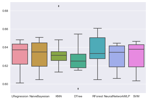
( Credits to Arun Prakash (Kaggle) for the very funny visualization )
let’s repeat it with other features (the team and the opponent)
rescaledX = rescaledX.join(marks_final[marks_final.columns[16:]])
rescaledX.head()
| LastMark | rankOpponentTeam | rankOwnTeam | playingHome | Atalanta | Cagliari | Cesena | Chievo | Empoli | Fiorentina | ... | Opp:Milan | Opp:Napoli | Opp:Palermo | Opp:Parma | Opp:Roma | Opp:Sampdoria | Opp:Sassuolo | Opp:Torino | Opp:Udinese | Opp:Verona | |
|---|---|---|---|---|---|---|---|---|---|---|---|---|---|---|---|---|---|---|---|---|---|
| 0 | -0.995670 | -0.058718 | -0.060266 | 1 | 1 | 0 | 0 | 0 | 0 | 0 | ... | 0 | 0 | 0 | 0 | 0 | 0 | 0 | 0 | 0 | 1 |
| 1 | 1.762298 | -0.058718 | -0.060266 | 0 | 1 | 0 | 0 | 0 | 0 | 0 | ... | 0 | 0 | 0 | 0 | 0 | 0 | 0 | 0 | 0 | 0 |
| 2 | 2.451790 | 0.824018 | -0.941649 | 1 | 1 | 0 | 0 | 0 | 0 | 0 | ... | 0 | 0 | 0 | 0 | 0 | 0 | 0 | 0 | 0 | 0 |
| 3 | 0.383314 | -0.764907 | -0.236543 | 0 | 1 | 0 | 0 | 0 | 0 | 0 | ... | 0 | 0 | 0 | 0 | 0 | 0 | 0 | 0 | 0 | 0 |
| 4 | 1.072806 | -1.647643 | 0.116011 | 1 | 1 | 0 | 0 | 0 | 0 | 0 | ... | 0 | 0 | 0 | 0 | 0 | 0 | 0 | 0 | 0 | 0 |
5 rows × 44 columns
X = rescaledX
X_train,X_test,Y_train,Y_test = train_test_split(X,Y, random_state = 42, test_size = 0.2)
results = []
names = []
for name,model in models:
    kfold = KFold(n_splits=10, random_state=42)
    cv_result = cross_val_score(model,X_train,Y_train, cv = kfold,scoring = "accuracy")
    names.append(name)
    results.append(cv_result)
for i in range(len(names)):
    print(names[i],results[i].mean())
('LRegression', 0.64243204427630651)
('NaiveBayesian', 0.57566490886163002)
('KNN', 0.68257114015310738)
('DTree', 0.64571662399531249)
('RForest', 0.66262689951214537)
('NeuralNetworkMLP', 0.68913186085317235)
('SVM', 0.63182630211318735)
ax = sns.boxplot(data=results)
ax.set_xticklabels(names)
plt.show()
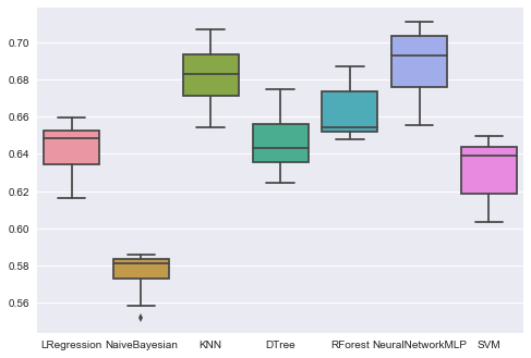
Knn and Neural Networks seems to be the most promising techniques. We have just tried them with their default configurations.
knn = KNeighborsClassifier()
knn.fit(X_train,Y_train)
predictions = knn.predict(X_test)
from sklearn.metrics import accuracy_score
from sklearn.metrics import classification_report
from sklearn.metrics import confusion_matrix
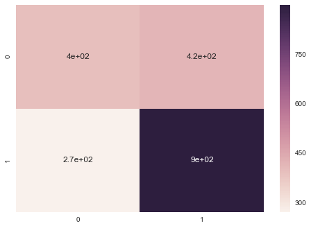
print(accuracy_score(Y_test,predictions))
0.653205451792
print(classification_report(Y_test,predictions))
             precision    recall  f1-score   support

          0       0.59      0.49      0.53       811
          1       0.68      0.77      0.72      1170

avg / total       0.65      0.65      0.65      1981
conf = confusion_matrix(Y_test,predictions)
label = ["0","1"]
sns.heatmap(conf, annot=True, xticklabels=label, yticklabels=label)
plt.show()
MLP = MLPClassifier()
MLP.fit(X_train,Y_train)
predictions = MLP.predict(X_test)
print(accuracy_score(Y_test,predictions))
0.668854114084
print(classification_report(Y_test,predictions))
             precision    recall  f1-score   support

          0       0.64      0.45      0.53       811
          1       0.68      0.82      0.75      1170

avg / total       0.66      0.67      0.66      1981
conf = confusion_matrix(Y_test,predictions)
label = ["0","1"]
sns.heatmap(conf, annot=True, xticklabels=label, yticklabels=label)
plt.show()
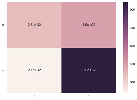
Not bad! .. To be continued