Quiz game data analysis
In this first data analysis, I will have fun analyzing the data from a quiz game. However, we will have access just to collection of the user feedbacks related to the questions.
Each record of the dataset represents a set of data for a single couple «question-answer»
- Information related to the question
- Information related to the answer and the feedback provided by the user during a game
Specifically, each record is characterized by the following features:
- Question ID : question identifier
- Category ID: category of the question
- Game ID: single game / match identifier
- Question Type: text / image question
- Answer : Correct / Wrong / Other
- Vote : feedback on the questions (thumb up / down)
import pandas as pd
import numpy as np
import matplotlib.pyplot as plt
from sklearn import preprocessing
votes = pd.read_csv('votes.csv') #to hide
categ = pd.read_csv('categories.csv',sep=';') #to hide!
votes = pd.merge(left = votes, right = categ, on= 'question_id')
votes.dropna(how='any', inplace=True)
Loading and cleaning. I know, dropping all these values can be aggressive. Maybe even here there is something interesting. Transform some of the data to facilitate some aggregated statistics.
def answers (code):
    if code == 0:
        return 1
    else:
        return 0

def answered (code):
    if code == 9:
        return 0
    else: return 1

def voteSimpl (vote):
    if vote==1:
        return 1
    else: return 0

def percentage (x,y):
    return float(x/float(y)*100)
votes['answerSimpl'] = map (lambda code: answers(code), votes['answer'])
votes['answered'] = map (lambda code: answered(code), votes['answer'])
votes['voteSimpl'] = map (lambda vote: voteSimpl(vote), votes['vote'])
let’s aggregate per question
quests = pd.DataFrame()
quests = votes.groupby('question_id', as_index=False).agg({"game_id": lambda x: x.count(), "user_id": lambda x: x.count(), "answered": np.sum, "answerSimpl": np.sum, "voteSimpl":  np.sum, "category_id": lambda x: x.iloc[0] }).reset_index()
quests.head()
| index | question_id | answerSimpl | user_id | answered | voteSimpl | game_id | category_id | |
|---|---|---|---|---|---|---|---|---|
| 0 | 0 | 1.0 | 49 | 72.0 | 72 | 57 | 72.0 | 1 |
| 1 | 1 | 2.0 | 21 | 28.0 | 28 | 24 | 28.0 | 1 |
| 2 | 2 | 3.0 | 22 | 40.0 | 40 | 32 | 40.0 | 1 |
| 3 | 3 | 4.0 | 30 | 53.0 | 53 | 37 | 53.0 | 1 |
| 4 | 4 | 5.0 | 26 | 32.0 | 31 | 24 | 32.0 | 1 |
quests['positivity'] = map ( lambda x,y: np.round(percentage(x,y),2), quests['voteSimpl'],quests['game_id'])
quests['correctness'] = map ( lambda x,y: np.round(percentage(x,y),2), quests['answerSimpl'],quests['game_id'])
quests['answer-ness'] = map ( lambda x,y: np.round(percentage(x,y),2), quests['answered'],quests['game_id'])
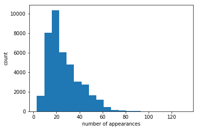
let’s have a look to the number of games (which is the number of appearances of each question)
print(quests['game_id'].mean())
plt.hist(quests['game_id'],bins=20)
plt.xlabel('number of appearances')
plt.ylabel('count')
#plt.savefig('hist_questions_games2.png', bbox_inches='tight')
plt.show()
26.3630126771
let us obtain some aggregated statistics
askedQuestions = pd.DataFrame()

askedQuestions = quests.ix[:, ['question_id','game_id']].sort_values('game_id', ascending=False)

#playedGames['agg_previous_value'] = playedGames['game_id'].shift(1) +  playedGames['game_id']

askedQuestions['agg_previous_value'] = askedQuestions['game_id'].cumsum()

askedQuestions['game_id_norm'] = (askedQuestions['game_id'] / float(askedQuestions['game_id'].sum())) * 100

#playedGames.ix[playedGames['game_id_norm'] < 0, 'game_id_norm'] = 0

askedQuestions['agg_previous_value_norm'] = askedQuestions['game_id_norm'].cumsum()

askedQuestions.head()
| question_id | game_id | agg_previous_value | game_id_norm | agg_previous_value_norm | |
|---|---|---|---|---|---|
| 6002 | 6560.0 | 132.0 | 132.0 | 0.012446 | 0.012446 |
| 3670 | 4118.0 | 117.0 | 249.0 | 0.011032 | 0.023478 |
| 5905 | 6452.0 | 115.0 | 364.0 | 0.010843 | 0.034321 |
| 3667 | 4115.0 | 108.0 | 472.0 | 0.010183 | 0.044504 |
| 3485 | 3918.0 | 107.0 | 579.0 | 0.010089 | 0.054593 |
askedQuestions.iloc[1]['agg_previous_value_norm']
0.023477631191871649
import matplotlib.ticker as mtick
import matplotlib.patches as patches

x = np.arange(1,len(askedQuestions['agg_previous_value_norm'])+1,1)
fig = plt.figure(1, (7,4))
ax = fig.add_subplot(1,1,1)
ax.plot(x,x*100/(len(askedQuestions['agg_previous_value_norm'])+1))
ax.plot(x,askedQuestions['agg_previous_value_norm'])

ax.add_patch(
    patches.Rectangle(
        (0, 0),
        #16832,
        len(askedQuestions['agg_previous_value_norm'])/10*4,
        #60.740781,
        askedQuestions.iloc[len(askedQuestions['agg_previous_value_norm'])/10*4]['agg_previous_value_norm'],
        fill=False,
        hatch='/'
    )
)

_ = plt.xlim(xmin=0, xmax=len(askedQuestions))
_ = plt.ylim(ymin=0, ymax=100)
ax.set_xticks(ticks=[len(askedQuestions)/4,len(askedQuestions)/4*2,len(askedQuestions)/4*3,len(askedQuestions)])
vals = ax.get_xticks()
ax.set_xticklabels(['{:3.2f}%'.format(float(x)/len(askedQuestions)*100) for x in vals])
plt.xlabel('Questions (sorted by number of appearances)')
plt.ylabel('Appearances (cumulative)')
#plt.savefig('questions_games_cumulative2.png', bbox_inches='tight')
plt.show()

very interesting, 60% of the occurrences are related to the top 40% questions!
print(quests['correctness'].mean())

plt.hist(quests['correctness'],bins=20)
plt.xlabel('correctness')
plt.ylabel('count')
#plt.savefig('hist_questions_correctness.png', bbox_inches='tight')
plt.show()
51.5491958737
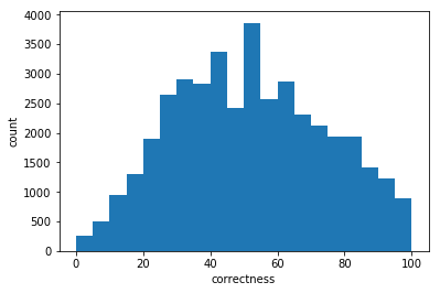
distribution of the correctness
print(quests['positivity'].mean())

plt.hist(quests['positivity'],bins=20)
plt.xlabel('positivity')
plt.ylabel('count')
#plt.savefig('hist_questions_positivity.png', bbox_inches='tight')
plt.show()
68.3658796918

Distribution of the positivity
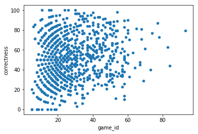
print(np.corrcoef( quests['game_id'],  quests['correctness'])[0, 1])

quests_sorted = quests.sort_values('game_id')
quests_sorted.plot.scatter('game_id','correctness')
plt.show()
0.154541271608

They appear more if they are correct: probably it was predictable (people can choose the category). The plot is a bit crowded.
print(np.corrcoef( quests['game_id'],  quests['correctness'])[0, 1])

quests_sorted = quests.sort_values('game_id')
quests_sorted.sample(1000).plot.scatter('game_id','correctness')
plt.show()
0.154541271608
print(np.corrcoef( quests['game_id'],  quests['positivity'])[0, 1])

quests_sorted = quests.sort_values('game_id')
quests_sorted.plot.scatter('game_id','positivity')
fit = np.polyfit(quests['game_id'], quests['positivity'], 1)
fit_fn = np.poly1d(fit)
plt.xlabel('appearances')
plt.plot(quests['game_id'], fit_fn(quests['game_id']), '--k')

#plt.savefig('corr_game_positivity.png', bbox_inches='tight')
plt.show()
0.150478799667
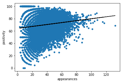
the positive questions appear more frequently! Maybe it is because of the same reason? or the system proposes the most appreciated?
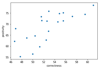
print(np.corrcoef( quests['correctness'],  quests['positivity'])[0, 1])

quests_sorted = quests.sample(10000).sort_values('correctness')
quests_sorted.plot.scatter('correctness','positivity')


fit = np.polyfit(quests['correctness'], quests['positivity'], 1)
fit_fn = np.poly1d(fit)
plt.xlabel('correctness')
plt.plot(quests['correctness'], fit_fn(quests['correctness']), '--k')

#plt.savefig('corr_correctness_positivity2.png', bbox_inches='tight')
plt.show()
0.48700343437
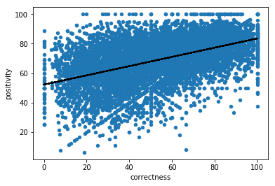
uh very interesting! people tend to like more the questions they know. Let us have a look at the type.
questsType = pd.DataFrame()
questsType = votes.groupby(['question_id', 'question_type'], as_index=False).agg({"game_id": lambda x: x.count(), "answered": np.sum, "answerSimpl": np.sum, "voteSimpl":  np.sum, "category_id": lambda x: x.iloc[0] }).reset_index()
questsType['positivity'] = map ( lambda x,y: np.round(percentage(x,y),2), questsType['voteSimpl'],questsType['game_id'])
questsType['correctness'] = map ( lambda x,y: np.round(percentage(x,y),2), questsType['answerSimpl'],questsType['game_id'])
questsType['answer-ness'] = map ( lambda x,y: np.round(percentage(x,y),2), questsType['answered'],questsType['game_id'])
questsType.head()
| index | question_id | question_type | game_id | category_id | answerSimpl | voteSimpl | answered | positivity | correctness | answer-ness | |
|---|---|---|---|---|---|---|---|---|---|---|---|
| 0 | 0 | 1.0 | 0.0 | 52.0 | 1 | 29 | 42 | 52 | 80.77 | 55.77 | 100.0 |
| 1 | 1 | 1.0 | 1.0 | 20.0 | 1 | 20 | 15 | 20 | 75.00 | 100.00 | 100.0 |
| 2 | 2 | 2.0 | 0.0 | 28.0 | 1 | 21 | 24 | 28 | 85.71 | 75.00 | 100.0 |
| 3 | 3 | 3.0 | 0.0 | 40.0 | 1 | 22 | 32 | 40 | 80.00 | 55.00 | 100.0 |
| 4 | 4 | 4.0 | 0.0 | 39.0 | 1 | 24 | 29 | 39 | 74.36 | 61.54 | 100.0 |
avgScoreMean = questsType['correctness'].mean()
avgScoreMedian = questsType['correctness'].median()
stdScore = questsType['correctness'].std()
print('avgScoreMean ' + str(avgScoreMean))
print('avgScoreMedian ' + str(avgScoreMedian))
print('stdScore '+ str(stdScore))
print('95% of the pop is between:')
print(np.percentile(questsType['correctness'], [2.5,97.5]))
avgScoreMean 51.9376343677
avgScoreMedian 50.0
stdScore 23.0419266109
95% of the pop is between:
[ 11.11  95.24]
Ok the avg is 50% but the interval is quite wide. Let’s have a look to the positivity, the correctness. Let’s have a look also to the answerness (people who just tried)
print(np.corrcoef( questsType['correctness'], questsType['positivity'])[0, 1])
questsType_sorted = questsType.head(1000).sort_values('correctness')
questsType_sorted.plot.scatter('correctness','positivity')
plt.show()
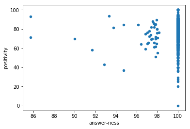
print(np.corrcoef( questsType['answer-ness'], questsType['positivity'])[0, 1])
questsType_sorted = questsType.head(1000).sort_values('answer-ness')
questsType_sorted.plot.scatter('answer-ness','positivity')
plt.show()
print(np.corrcoef( questsType['answer-ness'], questsType['correctness'])[0, 1])
questsType_sorted = questsType.head(1000).sort_values('answer-ness')
questsType_sorted.plot.scatter('answer-ness','correctness')
plt.show()
0.488562266626

0.00351013982096
0.0303497648239
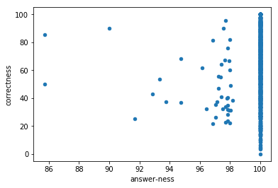
as before, high correlation between correctness and positivity.
avgScoreMean = questsType['positivity'].mean()
avgScoreMedian = questsType['positivity'].median()
stdScore = questsType['positivity'].std()
print('avgScoreMean ' + str(avgScoreMean))
print('avgScoreMedian ' + str(avgScoreMedian))
print('stdScore '+ str(stdScore))
print('95% of the pop is between:')
print(np.percentile(questsType['positivity'], [2.5,97.5]))
avgScoreMean 68.5143998004
avgScoreMedian 70.18
stdScore 14.7428556075
95% of the pop is between:
[ 35.71  92.86]
the positivity is quite high and steady. Let us understand it is biased by the type of questions
questsType0 = questsType[questsType['question_type'] ==0]
questsType1 = questsType[questsType['question_type'] ==1]
avgScoreMean = questsType0['correctness'].mean()
avgScoreMedian = questsType0['correctness'].median()
stdScore = questsType0['correctness'].std()
print('avgScoreMean ' + str(avgScoreMean))
print('avgScoreMedian ' + str(avgScoreMedian))
print('stdScore '+ str(stdScore))
print('95% of the pop is between:')
print(np.percentile(questsType0['correctness'], [2.5,97.5]))
avgScoreMean 51.4296481937
avgScoreMedian 50.0
stdScore 22.8260613194
95% of the pop is between:
[ 11.11  94.74]
avgScoreMean = questsType1['correctness'].mean()
avgScoreMedian = questsType1['correctness'].median()
stdScore = questsType1['correctness'].std()
print('avgScoreMean ' + str(avgScoreMean))
print('avgScoreMedian ' + str(avgScoreMedian))
print('stdScore '+ str(stdScore))
print('95% of the pop is between:')
print(np.percentile(questsType1['correctness'], [2.5,97.5]))
avgScoreMean 62.8929758713
avgScoreMedian 65.22
stdScore 24.8838536402
95% of the pop is between:
[  14.29  100.  ]
Ok it is clear how the questions of type1 are more easy to answer. Let us have a look at their feedbacks by the users
avgScoreMean = questsType0['positivity'].mean()
avgScoreMedian = questsType0['positivity'].median()
stdScore = questsType0['positivity'].std()
print('avgScoreMean ' + str(avgScoreMean))
print('avgScoreMedian ' + str(avgScoreMedian))
print('stdScore '+ str(stdScore))
print('95% of the pop is between:')
print(np.percentile(questsType0['positivity'], [2.5,97.5]))
avgScoreMean 68.328033117
avgScoreMedian 70.0
stdScore 14.6853248952
95% of the pop is between:
[ 35.71  92.31]
avgScoreMean = questsType1['positivity'].mean()
avgScoreMedian = questsType1['positivity'].median()
stdScore = questsType1['positivity'].std()
print('avgScoreMean ' + str(avgScoreMean))
print('avgScoreMedian ' + str(avgScoreMedian))
print('stdScore '+ str(stdScore))
print('95% of the pop is between:')
print(np.percentile(questsType1['positivity'], [2.5,97.5]))
avgScoreMean 72.5336246649
avgScoreMedian 75.0
stdScore 15.397627146
95% of the pop is between:
[  37.5  100. ]
Ok they are also slightly more appreciated. Good to know! now let’s look for something less generic. The difference between questions characterized of two types of representation and the ones only textual
def twoTypesQuest (question):
    if len(questsType[questsType["question_id"] == question])>1:
        return 1
    else: return 0

questsType['twoTypesQuest'] = map ( lambda question: twoTypesQuest (question), questsType['question_id'])
questsTypeText1type = questsType[(questsType['twoTypesQuest'] ==0) & (questsType['question_type'] ==0)]
questsTypeText2type = questsType[(questsType['twoTypesQuest'] ==1) & (questsType['question_type'] ==0)]
avgScoreMean = questsTypeText1type['correctness'].mean()
avgScoreMedian = questsTypeText1type['correctness'].median()
stdScore = questsTypeText1type['correctness'].std()
print('avgScoreMean ' + str(avgScoreMean))
print('avgScoreMedian ' + str(avgScoreMedian))
print('stdScore '+ str(stdScore))
print('95% of the pop is between:')
print(np.percentile(questsTypeText1type['correctness'], [2.5,97.5]))
avgScoreMean 51.0822332855
avgScoreMedian 50.0
stdScore 22.7389063427
95% of the pop is between:
[ 11.11  94.44]
avgScoreMean = questsTypeText2type['correctness'].mean()
avgScoreMedian = questsTypeText2type['correctness'].median()
stdScore = questsTypeText2type['correctness'].std()
print('avgScoreMean ' + str(avgScoreMean))
print('avgScoreMedian ' + str(avgScoreMedian))
print('stdScore '+ str(stdScore))
print('95% of the pop is between:')
print(np.percentile(questsTypeText2type['correctness'], [2.5,97.5]))
avgScoreMean 58.6109913793
avgScoreMedian 58.82
stdScore 23.438098832
95% of the pop is between:
[ 15.17625  97.83625]
Interestingly, the questions which can be expressed as a pictures are, generally more easy to understand and answer. Let us explore the positivity:
avgScoreMean = questsTypeText1type['positivity'].mean()
avgScoreMedian = questsTypeText1type['positivity'].median()
stdScore = questsTypeText1type['positivity'].std()
print('avgScoreMean ' + str(avgScoreMean))
print('avgScoreMedian ' + str(avgScoreMedian))
print('stdScore '+ str(stdScore))
print('95% of the pop is between:')
print(np.percentile(questsTypeText1type['positivity'], [2.5,97.5]))
avgScoreMean 68.1678410009
avgScoreMedian 70.0
stdScore 14.7072955975
95% of the pop is between:
[ 35.71  92.31]
avgScoreMean = questsTypeText2type['positivity'].mean()
avgScoreMedian = questsTypeText2type['positivity'].median()
stdScore = questsTypeText2type['positivity'].std()
print('avgScoreMean ' + str(avgScoreMean))
print('avgScoreMedian ' + str(avgScoreMedian))
print('stdScore '+ str(stdScore))
print('95% of the pop is between:')
print(np.percentile(questsTypeText2type['positivity'], [2.5,97.5]))
avgScoreMean 71.6393318966
avgScoreMedian 73.86
stdScore 13.8173123832
95% of the pop is between:
[ 38.58     92.81125]
As predictable, they are also more appreciated. However this is predictable as we have noticed a correlation between the correctness and the feedbacks. Focus now on categories
questsCat = pd.DataFrame()
questsCat = questsType.groupby(['category_id'], as_index=False).agg({"question_id": lambda x: x.nunique(), "game_id": np.sum, "answered": np.sum, "answerSimpl": np.sum, "voteSimpl":  np.sum}).reset_index()
questsCat['positivity'] = map ( lambda x,y: np.round(percentage(x,y),2), questsCat['voteSimpl'],questsCat['game_id'])
questsCat['correctness'] = map ( lambda x,y: np.round(percentage(x,y),2), questsCat['answerSimpl'],questsCat['game_id'])
questsCat['answer-ness'] = map ( lambda x,y: np.round(percentage(x,y),2), questsCat['answered'],questsCat['game_id'])

questsCat.head()
| index | category_id | game_id | answerSimpl | answered | voteSimpl | question_id | positivity | correctness | answer-ness | |
|---|---|---|---|---|---|---|---|---|---|---|
| 0 | 0 | #SKIP# | 199.0 | 162 | 199 | 147 | 9.0 | 73.87 | 81.41 | 100.00 |
| 1 | 1 | 1 | 58193.0 | 33288 | 58109 | 42802 | 1261.0 | 73.55 | 57.20 | 99.86 |
| 2 | 2 | 10 | 74034.0 | 45208 | 73920 | 58143 | 1372.0 | 78.54 | 61.06 | 99.85 |
| 3 | 3 | 11 | 51731.0 | 26075 | 51662 | 33458 | 3507.0 | 64.68 | 50.40 | 99.87 |
| 4 | 4 | 12 | 42914.0 | 20035 | 42853 | 26710 | 3403.0 | 62.24 | 46.69 | 99.86 |
Discard, for now, these categories
questsCat = questsCat[questsCat['category_id'] != '#SKIP#']
questsCat = questsCat[questsCat['category_id'] != 'Null']
avgScoreMean = questsCat['question_id'].mean()
avgScoreMedian = questsCat['question_id'].median()
stdScore = questsCat['question_id'].std()
print('avgScoreMean ' + str(avgScoreMean))
print('avgScoreMedian ' + str(avgScoreMedian))
print('stdScore '+ str(stdScore))
print('95% of the pop is between:')
print(np.percentile(questsCat['question_id'], [2.5,97.5]))
avgScoreMean 2003.55
avgScoreMedian 1879.0
stdScore 834.669520166
95% of the pop is between:
[ 1013.675  3562.125]
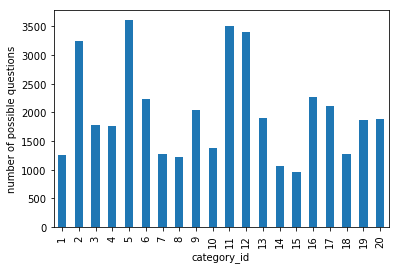
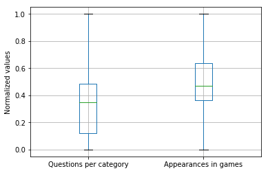
The categories are very unbalanced.
print(questsCat['question_id'].mean())

questsCat['category_id'] = map (lambda x: int(x), questsCat['category_id'])
_ = questsCat.sort_values('category_id').plot.bar(y='question_id', x='category_id')
plt.ylabel('number of possible questions')
_.legend_.remove()
#plt.savefig('plot_category_questions.png', bbox_inches='tight')
plt.show()
2003.55
avgScoreMean = questsCat['game_id'].mean()
avgScoreMedian = questsCat['game_id'].median()
stdScore = questsCat['game_id'].std()
print('avgScoreMean ' + str(avgScoreMean))
print('avgScoreMedian ' + str(avgScoreMedian))
print('stdScore '+ str(stdScore))
print('95% of the pop is between:')
print(np.percentile(questsCat['game_id'], [2.5,97.5]))
avgScoreMean 52849.6
avgScoreMedian 51803.0
stdScore 12844.3257404
95% of the pop is between:
[ 29295.225  76526.7  ]
Their distribution in the games, instead is more uniform
np.corrcoef( questsCat['game_id'], questsCat['question_id'])[0, 1]
0.06246680003354263
avgScoreMean = questsCat['correctness'].mean()
avgScoreMedian = questsCat['correctness'].median()
stdScore = questsCat['correctness'].std()
print('avgScoreMean ' + str(avgScoreMean))
print('avgScoreMedian ' + str(avgScoreMedian))
print('stdScore '+ str(stdScore))
print('95% of the pop is between:')
print(np.percentile(questsCat['correctness'], [2.5,97.5]))
avgScoreMean 52.701
avgScoreMedian 52.51
stdScore 3.89205520056
95% of the pop is between:
[ 46.78025  60.32375]
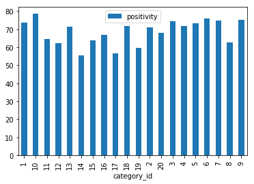
avgScoreMean = questsCat['positivity'].mean()
avgScoreMedian = questsCat['positivity'].median()
stdScore = questsCat['positivity'].std()
print('avgScoreMean ' + str(avgScoreMean))
print('avgScoreMedian ' + str(avgScoreMedian))
print('stdScore '+ str(stdScore))
print('95% of the pop is between:')
print(np.percentile(questsCat['positivity'], [2.5,97.5]))
avgScoreMean 68.5655
avgScoreMedian 71.235
stdScore 6.7528305761
95% of the pop is between:
[ 55.8805  77.267 ]
Their correctness and positivity, is instead, very balanced
_ = questsCat.plot.bar(y='positivity', x='category_id')
plt.show()
min_max_scaler = preprocessing.MinMaxScaler()
questsCat['question_id_norm'] = min_max_scaler.fit_transform(questsCat['question_id'])
questsCat['game_id_norm'] = min_max_scaler.fit_transform(questsCat['game_id'])

_ = questsCat.boxplot(['positivity', 'correctness'])
plt.show()
#not interesting


_ = questsCat.boxplot(['question_id_norm', 'game_id_norm'])
plt.ylabel('Normalized values')
plt.xticks([1, 2], ['Questions per category', 'Appearances in games'])
#plt.savefig('distr_category_questions_games.png', bbox_inches='tight')
plt.show()
plt.show()

print(np.corrcoef( questsCat['game_id'],  questsCat['positivity'])[0, 1])

fit = np.polyfit(questsCat['game_id'], questsCat['positivity'], 1)
fit_fn = np.poly1d(fit)


questsCatSorted = questsCat.sort_values('game_id')
questsCatSorted.plot.scatter('game_id','positivity')

plt.xlabel('number of appearances in games (categories)')

plt.plot(questsCat['game_id'], fit_fn(questsCat['game_id']), '--k')
#plt.savefig('corr_positivity_games.png', bbox_inches='tight')
plt.show()
0.628175927796
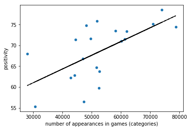
The system is already using a recc system to propose the most appreciated questions. Or, instead the people just select the categories they love more. So they are more appreciated and also more “played”
print(np.corrcoef( questsCat['game_id'],  questsCat['question_id'])[0, 1])

questsCatSorted = questsCat.sort_values('question_id')
questsCatSorted.plot.scatter('question_id','game_id')

plt.xlabel('number of possible questions (categories)')
plt.ylabel('Appearances in games')
#plt.savefig('corr_questions_games.png', bbox_inches='tight')
plt.show()
0.0624668000335
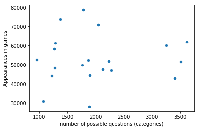
no relationship between the the question per category and the categories appearances
print(np.corrcoef( questsCat['correctness'],  questsCat['positivity'])[0, 1])

questsCatSorted = questsCat.sort_values('correctness')
questsCatSorted.plot.scatter('correctness','positivity')

plt.show()
0.732173457654
very predictable, as before: positive only if they answer correctly
let’s aggregate per game
games = votes.groupby(['game_id'], as_index=False).agg({"user_id": lambda x: x.nunique(), "question_id": lambda x: x.count(), "answered": np.sum, "answerSimpl": np.sum, "voteSimpl":  np.sum, 'question_type' : np.sum })
games['game_id'].nunique()
539198
games['positivity'] = map ( lambda x,y: np.round(percentage(x,y),2), games['voteSimpl'],games['question_id'])
games['correctness'] = map ( lambda x,y: np.round(percentage(x,y),2), games['answerSimpl'],games['question_id'])
games['answer-ness'] = map ( lambda x,y: np.round(percentage(x,y),2), games['answered'],games['question_id'])
games['picture-ness'] = map ( lambda x,y: np.round(percentage(x,y),2), games['question_type'],games['question_id'])
print(len(games))
print(games.ix[games['user_id'] == 2, 'question_id'].mean())
print(len(games[games['user_id'] == 2]))
print(len(games[games['user_id'] == 2])/float(len(games))*100)
plt.hist(games.ix[games['user_id'] == 2, 'question_id'],bins=10)

plt.xlabel('number of questions')
plt.ylabel('count')
plt.savefig('games_questions2.png', bbox_inches='tight')
plt.show()
539198
3.57255630369
64605
11.9816839083
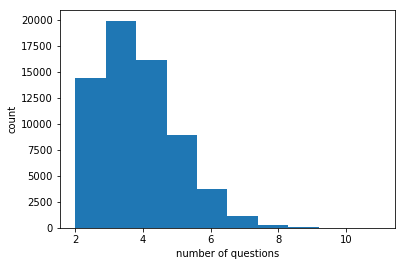
Some games are played by just 1 player!
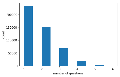
print(games.ix[games['user_id'] == 1, 'question_id'].mean())

print(len(games[games['user_id'] == 1]))
print(len(games[games['user_id'] == 1])/float(len(games))*100)

plt.hist(games.ix[games['user_id'] == 1, 'question_id'],bins=10)

plt.xlabel('number of questions')
plt.ylabel('count')
plt.savefig('games_questions1.png', bbox_inches='tight')
plt.show()
1.74840126171
474593
88.0183160917
plt.hist(games['question_id'],bins=10)

plt.xlabel('number of questions')
plt.ylabel('games count')
plt.savefig('games_questions_all.png', bbox_inches='tight')
plt.show()

This is very strange: some games have 2 players while some others has 1. the only explanation I can think about is that there are just the data about the rated questions, which, maybe are a few per games. Hence this data are not suggested to extract statistics related to games, but, still can be useful for questions and users informations.
let’s aggregate per user
users = votes.groupby(['user_id'], as_index=False).agg({"game_id": lambda x: x.nunique(), "question_id": lambda x: x.count(), "answered": np.sum, "answerSimpl": np.sum, "voteSimpl": np.sum, 'question_type' : np.sum }).reset_index()
users['positivity'] = map ( lambda x,y: np.round(percentage(x,y),2), users['voteSimpl'],users['question_id'])
users['correctness'] = map ( lambda x,y: np.round(percentage(x,y),2), users['answerSimpl'],users['question_id'])
users['answer-ness'] = map ( lambda x,y: np.round(percentage(x,y),2), users['answered'],users['question_id'])
users.head()
| index | user_id | answerSimpl | answered | voteSimpl | question_type | game_id | question_id | positivity | correctness | answer-ness | |
|---|---|---|---|---|---|---|---|---|---|---|---|
| 0 | 0 | 12.0 | 0 | 0 | 1 | 0.0 | 1.0 | 1.0 | 100.0 | 0.00 | 0.0 |
| 1 | 1 | 63.0 | 2 | 4 | 4 | 1.0 | 4.0 | 4.0 | 100.0 | 50.00 | 100.0 |
| 2 | 2 | 407.0 | 60 | 85 | 68 | 2.0 | 44.0 | 85.0 | 80.0 | 70.59 | 100.0 |
| 3 | 3 | 706.0 | 1 | 3 | 3 | 0.0 | 1.0 | 3.0 | 100.0 | 33.33 | 100.0 |
| 4 | 4 | 718.0 | 1 | 2 | 1 | 0.0 | 1.0 | 2.0 | 50.0 | 50.00 | 100.0 |
print(users['question_id'].mean())
print(users['game_id'].mean())
18.4468640206
10.5020176018
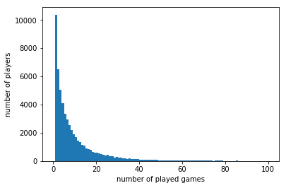
plt.hist(users['game_id'],bins=100, range=(0, 100))
plt.xlabel('number of played games')
plt.ylabel('number of players')
plt.savefig('hist_played_games_0-100.png', bbox_inches='tight')
plt.show()

len(users[users['game_id'] == 1]) / float(len(users)) * 100
18.041882631231086
(len(users[users['game_id'] <=3]))/ float(len(users)) * 100
38.181375447872824
let us explore correlations
np.corrcoef(users['game_id'],users['question_id'])[0,1]
0.98969409280107545
np.corrcoef(users['correctness'],users['question_id'])[0,1]
0.0064310028086971569
users.sample(10000).plot.scatter('correctness','question_id')
plt.savefig('corr_question_correctness.png', bbox_inches='tight')
plt.ylabel('number of answered questions')
plt.xlabel('percentage of correct answers')
plt.savefig('corr_question_correctness.png', bbox_inches='tight')

plt.show()

np.corrcoef(users['positivity'],users['question_id'])[0,1]
0.10247536990881757
users.sample(10000).plot.scatter('positivity','question_id')
plt.ylabel('number of answered questions')
plt.xlabel('percentage of appreciated questions')
plt.savefig('corr_question_positivity.png', bbox_inches='tight')

plt.show()
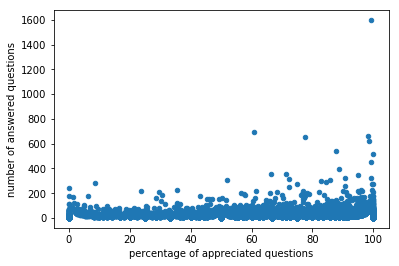
they are not discouraged! the positivity seems more effective though
the statistics about the questions are very similar
plt.hist(users['question_id'],bins=100, range=(0, 100))

plt.xlabel('number of answered questions')
plt.ylabel('number of players')
plt.savefig('hist_answered_question_0-100.png', bbox_inches='tight')
plt.show()
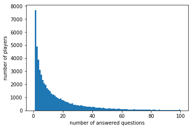
(len(users[users['question_id'] <=5]))/ float(len(users)) * 100
38.790134622743246
Lot of players with less than 5 questions answered
plt.hist(users['game_id'],bins=100, range=(0, 100))

plt.xlabel('number of played games')
plt.ylabel('number of players')
plt.savefig('hist_played_games_0-100.png', bbox_inches='tight')
plt.show()
Almost 1 rated question per answer. Let’s obtain some aggregated statistics
playedGames = pd.DataFrame()

playedGames = users.ix[:, ['user_id','game_id']].sort_values('game_id', ascending=False)

#playedGames['agg_previous_value'] = playedGames['game_id'].shift(1) +  playedGames['game_id']

playedGames['agg_previous_value'] = playedGames['game_id'].cumsum()

playedGames['game_id_norm'] = (playedGames['game_id'] / float(playedGames['game_id'].sum())) * 100

#playedGames.ix[playedGames['game_id_norm'] < 0, 'game_id_norm'] = 0

playedGames['agg_previous_value_norm'] = playedGames['game_id_norm'].cumsum()

playedGames.head()
| user_id | game_id | agg_previous_value | game_id_norm | agg_previous_value_norm | |
|---|---|---|---|---|---|
| 46798 | 1.099269e+09 | 852.0 | 852.0 | 0.141106 | 0.141106 |
| 12460 | 1.714551e+06 | 727.0 | 1579.0 | 0.120404 | 0.261509 |
| 20817 | 2.226343e+06 | 628.0 | 2207.0 | 0.104007 | 0.365517 |
| 32482 | 3.164324e+06 | 577.0 | 2784.0 | 0.095561 | 0.461078 |
| 12127 | 1.695558e+06 | 559.0 | 3343.0 | 0.092580 | 0.553657 |
import matplotlib.ticker as mtick
import matplotlib.patches as patches

x = np.arange(1,len(playedGames['agg_previous_value_norm'])+1,1)
fig = plt.figure(1, (7,4))
ax = fig.add_subplot(1,1,1)
ax.plot(x,x*100/(len(playedGames['agg_previous_value_norm'])+1))
ax.plot(x,playedGames['agg_previous_value_norm'])

ax.add_patch(
    patches.Rectangle(
        (0, 0),
        17608,
        75.000372,
        fill=False,
        hatch='/'
  )
)

_ = plt.xlim(xmin=0, xmax=57524)
_ = plt.ylim(ymin=0, ymax=100)
ax.set_xticks(ticks=[57524/4,57524/4*2,57524/4*3,57524])
vals = ax.get_xticks()
ax.set_xticklabels(['{:3.2f}%'.format(float(x)/57524*100) for x in vals])
plt.xlabel('Players (sorted by number of games played)')
plt.ylabel('Played Games (cumulative)')
plt.savefig('users_games.png', bbox_inches='tight')
plt.show()
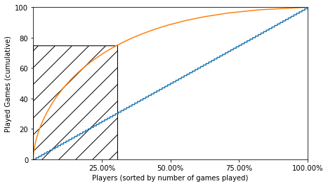
30% of the users player 75% of the games. This is huge! very similar behavior with the questions
playedQuestion = pd.DataFrame()

playedQuestion = users.ix[:, ['user_id','question_id']].sort_values('question_id', ascending=False)

#playedGames['agg_previous_value'] = playedGames['game_id'].shift(1) +  playedGames['game_id']

playedQuestion['agg_previous_value'] = playedQuestion['question_id'].cumsum()

playedQuestion['question_id_norm'] = (playedQuestion['question_id'] / float(playedQuestion['question_id'].sum())) * 100

playedQuestion.ix[playedQuestion['question_id_norm'] < 0, 'question_id_norm'] = 0

playedQuestion['agg_previous_value_norm'] = playedQuestion['question_id_norm'].cumsum()

playedQuestion.head()
| user_id | question_id | agg_previous_value | question_id_norm | agg_previous_value_norm | |
|---|---|---|---|---|---|
| 46798 | 1.099269e+09 | 1596.0 | 1596.0 | 0.150483 | 0.150483 |
| 12460 | 1.714551e+06 | 1261.0 | 2857.0 | 0.118897 | 0.269380 |
| 20817 | 2.226343e+06 | 1142.0 | 3999.0 | 0.107677 | 0.377056 |
| 32482 | 3.164324e+06 | 1077.0 | 5076.0 | 0.101548 | 0.478604 |
| 12127 | 1.695558e+06 | 1029.0 | 6105.0 | 0.097022 | 0.575626 |
playedQuestion['question_id'].mean()
18.446864020593452
import matplotlib.ticker as mtick
import matplotlib.patches as patches
x = np.arange(1,len(playedQuestion['agg_previous_value_norm'])+1,1)
fig = plt.figure(1, (7,4))
ax = fig.add_subplot(1,1,1)
ax.plot(x,x*100/(len(playedQuestion['agg_previous_value_norm'])+1))
ax.plot(x,playedQuestion['agg_previous_value_norm'])
ax.add_patch(
patches.Rectangle(
(0, 0),
16175,
75.000372,
fill=False,
hatch='/'
)
)
_ = plt.xlim(xmin=-100, xmax=57524)
_ = plt.ylim(ymin=0, ymax=100)
ax.set_xticks(ticks=[57524/4,57524/4*2,57524/4*3,57524])
vals = ax.get_xticks()
ax.set_xticklabels(['{:3.2f}%'.format(float(x)/57524*100) for x in vals])
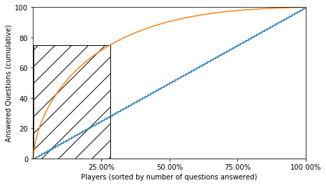
plt.xlabel('Players (sorted by number of questions answered)')
plt.ylabel('Answered Questions (cumulative)')
plt.savefig('users_questions.png', bbox_inches='tight')
plt.show()
users['positivePerGame'] = map ( lambda x,y: np.round(x/float(y),2), users['voteSimpl'],users['game_id'])
users['correctPerGame'] = map ( lambda x,y: np.round(x/float(y),2), users['answerSimpl'],users['game_id'])
users['answerPerGame'] = map ( lambda x,y: np.round(x/float(y),2), users['answered'],users['game_id'])
users['positivityTotal'] = map ( lambda x,y: np.round(percentage(x,y),2), users['voteSimpl'],users['question_id'])
users['correctnessTotal'] = map ( lambda x,y: np.round(percentage(x,y),2), users['answerSimpl'],users['question_id'])
users['answer-nessTotal'] = map ( lambda x,y: np.round(percentage(x,y),2), users['answered'],users['question_id'])
users.head()
| index | user_id | answerSimpl | answered | voteSimpl | question_type | game_id | question_id | positivity | correctness | answer-ness | positivePerGame | correctPerGame | answerPerGame | positivityTotal | correctnessTotal | answer-nessTotal | |
|---|---|---|---|---|---|---|---|---|---|---|---|---|---|---|---|---|---|
| 0 | 0 | 12.0 | 0 | 0 | 1 | 0.0 | 1.0 | 1.0 | 100.0 | 0.00 | 0.0 | 1.00 | 0.00 | 0.00 | 100.0 | 0.00 | 0.0 |
| 1 | 1 | 63.0 | 2 | 4 | 4 | 1.0 | 4.0 | 4.0 | 100.0 | 50.00 | 100.0 | 1.00 | 0.50 | 1.00 | 100.0 | 50.00 | 100.0 |
| 2 | 2 | 407.0 | 60 | 85 | 68 | 2.0 | 44.0 | 85.0 | 80.0 | 70.59 | 100.0 | 1.55 | 1.36 | 1.93 | 80.0 | 70.59 | 100.0 |
| 3 | 3 | 706.0 | 1 | 3 | 3 | 0.0 | 1.0 | 3.0 | 100.0 | 33.33 | 100.0 | 3.00 | 1.00 | 3.00 | 100.0 | 33.33 | 100.0 |
| 4 | 4 | 718.0 | 1 | 2 | 1 | 0.0 | 1.0 | 2.0 | 50.0 | 50.00 | 100.0 | 1.00 | 1.00 | 2.00 | 50.0 | 50.00 | 100.0 |
let’s mine other info about the user
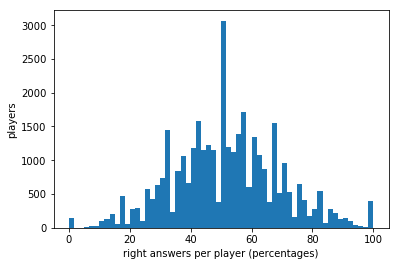
print(users['correctness'].mean())

plt.hist(users['correctness'],bins=20)

plt.xlabel('right answers per player (percentages)')
plt.ylabel('players')
plt.savefig('hist_correctness_0-100.png', bbox_inches='tight')
plt.show()
53.0714472815

print(users['positivity'].mean())

plt.hist(users['positivity'],bins=20)

plt.xlabel('fraction of answers positively rated')
plt.ylabel('players')
plt.savefig('hist_positively_0-100.png', bbox_inches='tight')
plt.show()
63.0030728424

try to understand which is the impact of the newbies
usersSerious= users[users['question_id']>5]
usersNewbies= users[users['question_id']<=5]
print(usersSerious['correctness'].mean())

plt.hist(usersSerious['correctness'],bins=60)

plt.xlabel('right answers per player (percentages)')
plt.ylabel('players')
plt.savefig('hist_correctnessSerious_0-100.png', bbox_inches='tight')
plt.show()
51.6071246306
print(usersSerious['positivity'].mean())

plt.hist(usersSerious['positivity'],bins=20)

plt.xlabel('fraction of answers positively rated')
plt.ylabel('players')
plt.savefig('hist_positiveSerious_0-100.png', bbox_inches='tight')
plt.show()
66.1663071153

way better, even if I suspect there are some cheaters =)
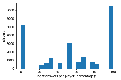
print(usersNewbies['correctness'].mean())

plt.hist(usersNewbies['correctness'],bins=20)

plt.xlabel('right answers per player (percentage)s')
plt.ylabel('players')
plt.savefig('hist_correctnessNewbies_0-100.png', bbox_inches='tight')
plt.show()
55.3821119182
print(usersNewbies['positivity'].mean())

plt.hist(usersNewbies['positivity'],bins=20)

plt.xlabel('right answers per player (percentage)s')
plt.ylabel('players')
plt.savefig('hist_positivityNewbies_0-100.png', bbox_inches='tight')
plt.show()
58.0115680208
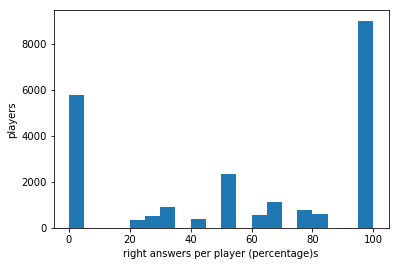
Ok, the newbies seem to be better players than more experience player. The distribution is very different and it is clear that this has not happened by chance. However, just to “show-off” a bit, let’s see what we could have done to understand if it has happened by chance. We will use a permutation based statistical hypothesis testing (A/B test). Before proceeding, let’s prepare our tools: - the function to deliver the permutation of the two sets - the function to deliver the measured statistics of the permutations - a modified mean function, since the usual permutation replicate function needs a function with 2 arguments as input
from __future__ import division
def permutation_sample(data1, data2):
    """Generate a permutation sample from two data sets."""
    data = np.concatenate((data1,data2),)
    permuted_data = np.random.permutation(data)
    perm_sample_1 = permuted_data[:len(data1)]
    perm_sample_2 = permuted_data[len(data1):]
    return perm_sample_1, perm_sample_2

def draw_perm_reps(data_1, data_2, func, size=1):
    """Generate multiple permutation replicates."""

    perm_replicates = np.empty(size)
    for i in range(size):
        perm_sample_1, perm_sample_2 = permutation_sample(data_1,data_2)
        # Compute the test statistic
        perm_replicates[i] = func(perm_sample_1,perm_sample_2)
    return perm_replicates

def mean4perm(data1, data2):
    """mean of the first data"""
    m = np.sum(data1) / len(data1)
    return m
print(usersNewbies['correctness'].mean())
print(usersSerious['correctness'].mean())
55.3821119182
51.6071246306
My null ipothesis is that the number of answered question do not affect the correctness. Let’s misurate which is the probability to have a more extreme (higher in this case) correctness mean with a permutation test. Our threshold (Alpha) will be 0.05, corresponding to include the 95% of the population. If our p values will be under this threshold, we will reject the null hypothesis.
from __future__ import division


perm_replicates = draw_perm_reps(usersNewbies['correctness'], usersSerious['correctness'], mean4perm, 10000)

p = np.sum(perm_replicates >= usersNewbies['correctness'].mean()) / len(perm_replicates)
print('p-value = '+str(p))
p-value = 0.0
As expected, since the data distributions were very different from each other, the p-value is very low (0!) and, hece, very significant. We definetely reject the null hypothesis (the distribution of the correct answers is not affected by the number of played games)
What else we can do with the data we have? Since we have seen how appreciation is one of the factor pushing people to keep playing, why don’t we think about something to increase the positivity? Something to propose the users the question they like? Let’s have a look to a naive implementation of a Recommendation System based on frequent itemset mining and association rule. This technique is a very popular data mining tool used to extract correlation and rules in => then. We will use this to propose the users some questions on the basis on their previous likes.
import csv

votes=votes[votes['vote'] == 1]
userDict = {}

for user in votes['user_id'].drop_duplicates():
    questions = list(votes.ix[votes['user_id']==user,'question_id'].drop_duplicates())
    userDict[user]=questions

with open('dict.csv', 'wb') as csv_file:
    writer = csv.writer(csv_file)
    for key, value in userDict.items():
       writer.writerow(value)
write the dictionary to a csv file. In this way, we are able to apply a common frequent itemset and association rules miner. I have used the Eclat implementation by Christian Borgelt but there are plenty of them.
Import now the obtained rules. We have also obtained the occurrences of each question. In this way, we are also able to propose the most appreciated questions in case the rec system is not able to propose something ad hoc for the user.
freq = pd.read_csv('freq.csv', header=None)
rules = pd.read_csv('rules_classic.csv', header=None)
rules.columns = ['then','if','supp','conf']
freq.columns = ['question_id','supp']
rules.head()
| then | if | supp | conf | |
|---|---|---|---|---|
| 0 | 38255 | 6704 | 0.015882 | 50.0 |
| 1 | 19173 | 38136 | 0.011911 | 50.0 |
| 2 | 13345 | 14621 | 0.011911 | 50.0 |
| 3 | 9930 | 32825 | 0.011911 | 50.0 |
| 4 | 12423 | 29149 | 0.011911 | 50.0 |
freq.head()
| question_id | supp | |
|---|---|---|
| 0 | 3918 | 0.188597 |
| 1 | 58 | 0.182641 |
| 2 | 6560 | 0.180656 |
| 3 | 6452 | 0.170730 |
| 4 | 1062 | 0.168745 |
reorder the columns (i like the if before the then on the left!)
cols = rules.columns.tolist()
cols.remove('if')
cols.insert(0,'if')
cols
['if', 'then', 'supp', 'conf']
rules = rules[cols]
rules = rules.sort_values(['supp','conf'], ascending = False)
rules['if'] = map(lambda x: int(x), rules['if'])
rules['then'] = map(lambda x: int(x), rules['then'])
rules.head()
| if | then | supp | conf | |
|---|---|---|---|---|
| 0 | 6704 | 38255 | 0.015882 | 50.0 |
| 1 | 38136 | 19173 | 0.011911 | 50.0 |
| 2 | 14621 | 13345 | 0.011911 | 50.0 |
| 3 | 32825 | 9930 | 0.011911 | 50.0 |
| 4 | 29149 | 12423 | 0.011911 | 50.0 |
Let’s create an example for which we know the desired output. Select 1 player and add to his history two questions: one is in the if value and the second is the very first suggested question of that specific rule. The ‘engine’ should propose the second in line question for that user (in this case they all have the same support and confidence so it just take the first, but the system should select the most reliable (support and confidence) one in general).
#let's imagine a player with his historic collection of liked questions

playerId = 3.673360e+05

questionsPlayer = np.array(votes.ix[votes['user_id'] == 3.673360e+05, 'question_id'].values)
questionsPlayer = np.append(questionsPlayer, 22386)
questionsPlayer = np.append(questionsPlayer, 4358)

questionsPlayer
array([ 21691.,  30762.,  17657.,   6396.,  14403.,   6566.,  34752.,
        24282.,   7640.,  19430.,  15943.,  23899.,   3147.,  31444.,
        40463.,  10469.,   9546.,  40570.,  41865.,  23239.,  30825.,
         9295.,   9633.,  22386.,   4358.])
rules[(rules['if'] == 4358)]
| if | then | supp | conf | |
|---|---|---|---|---|
| 227 | 4358 | 22386 | 0.007941 | 50.0 |
| 228 | 4358 | 31313 | 0.007941 | 50.0 |
| 229 | 4358 | 41631 | 0.007941 | 50.0 |
| 230 | 4358 | 29024 | 0.007941 | 50.0 |
| 231 | 4358 | 23814 | 0.007941 | 50.0 |
# questionsPlayer = liked question
def Rec (questionsPlayer):
    """Propose, if possible, a question based on the history of the rates"""
    found = False


    #analyze the history, starting from the last appreciated question
    questionsPlayer = questionsPlayer[::-1]

    for question in questionsPlayer:
        if (found): break
        if int(question) in rules['if'].values:    #look through the rules if column
            proposed = rules.ix[rules['if'] == question, 'then'].values
            for proposedQuestion in proposed:
                if (found): break
                if (proposedQuestion not in questionsPlayer): #it should not be repated
                    #of course, a more advanced engine would try to avoid the not like questions
                    print ('proposed question: '+str(proposedQuestion))
                    found = True
                    break
    #if it was not possible to exploit the history, let's propose the most appreciated one
    if (found == False): #it means that there were no rules
        for proposedQuestion in freq['question_id']: #rules are already sorted
            if (proposedQuestion not in questionsPlayer):
                print ('proposed question: '+str(proposedQuestion))
                found = True
                break
    #no suggestions, sorry
    if (found == False):
        print('sorry, no suggestions')