AB-Testing
We are developing and managing our fitness mobile application. Each new feature should be carefully developed and tested. Let’s image we want to test the impact on the loading time of a new feature and we have just 24h to test it.
Before the start of the hypothesis testing, we should generate our dummy data.
Focus initially on the social feed loading time. Since the test is very short (24h), we disclose the new feature for half of the users. In this way, at the same time, we are not biasing the analysis with different loading time related to the number of users using the server. Indeed, if we consider just a small amount of users, there is the possibility that the additional loading time is not realistic because the central server is not much loaded.
Therefore, is half of the active users. Is a quite high number but 24h is a very short period to obtain accurate measures.
Let’s start with something easy. Imagine that we have already the loading time distribution among the users. We know the feature has been disclosed for half of the users. So we have two distributions, the first related to the normal users, and the second related to the users trying the new feature.
I decided to model it with a lognorm distribution, which is often used to model server waiting time. It is the log of a normal distribution. We could have modeled it with a more simple uniform distribution.
The social feed is usually loaded in about 1 second. let’s assume a variance value up to 0.3s.
Let us assume that the feature is related to a new functionality or content (i.e. not related to the algorithm used to load the social feature). Therefore, in our dummy data, we increase a bit the loading time average and the variance.
import numpy as np
import pandas as pd
import scipy.stats as stats
from scipy.stats import lognorm
import matplotlib.pyplot as plt
import math
import seaborn as sns
r = np.random.lognormal(mean=np.log(1),sigma=0.3, size = 12500) #performant devices
r1 = np.random.lognormal(mean=np.log(1.5),sigma=0.3, size = 12500)  #old devices
r = np.concatenate([r,r1])

feature = np.random.lognormal(mean=np.log(1),sigma=0.3, size = 12500) #performant devices
feature1 = np.random.lognormal(mean=np.log(1.52),sigma=0.32, size = 12500) #old devices
feature = np.concatenate([feature,feature1])

bins = np.linspace(0, 4, 50)

plt.hist(r, bins, alpha=0.5, normed = True, label='no feature')
plt.hist(feature, bins, alpha=0.5, normed = True, label='with feature')
plt.legend(loc='upper right')
_ = plt.xlabel('loading time (seconds)')
_ = plt.ylabel('Number of users (Normalized - PDF)')
plt.savefig('distributionsLogNorm.png', bbox_inches='tight')
plt.show()
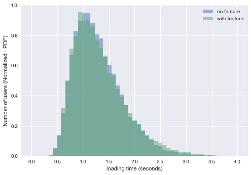
We can see how the two distributions are very similar. The distribution of the SFLT of the users with the feature is a bit more spread after the zero. The users without the new feature are experience a more steady waiting time in the social feed.
These are the means of our distributions. The second one is higher. We know that it has not happened by chance because we have created it different. However, in a real scenario, what can we say about it? Is it statistically significant? which is the probability that this difference just happend by chance? 95% of the population is spread between approximately 0.6s and 2.5 - 2.6s (depending if the feature is adopted). These are our Y-Z values
print(r.mean())
print(feature.mean())
1.30754011149
1.32553125788
perc = np.percentile(r, [2.5, 97.5])
print(perc)

perc = np.percentile(feature, [2.5, 97.5])
print(perc)
[ 0.60946619  2.44958572]
[ 0.60491894  2.58996936]
Let’s import my personal toolkit for statistical hypothesis testing. In this case we will run a two-sample permutation-based hypothesis test. This is used for testing differences between independent groups.
#statistical hypothesis testing toolkit

from __future__ import division
def permutation_sample(data1, data2):
    """Generate a permutation sample from two data sets."""
    data = np.concatenate((data1,data2),)
    permuted_data = np.random.permutation(data)
    perm_sample_1 = permuted_data[:len(data1)]
    perm_sample_2 = permuted_data[len(data1):]
    return perm_sample_1, perm_sample_2

def draw_perm_reps(data_1, data_2, func, size=1):
    """Generate multiple permutation replicates."""
    perm_replicates = np.empty(size)
    for i in range(size):
        perm_sample_1, perm_sample_2 = permutation_sample(data_1,data_2)
        # Compute the test statistic
        perm_replicates[i] = func(perm_sample_1,perm_sample_2)
    return perm_replicates

def mean4perm(data1, data2):
    """mean of the first data"""
    m = np.sum(data1) / len(data1)
    return m
Our null hypothesis states there is no difference in the loading time. We set a threshold of 95% of confidence. Our test statistic is the mean of the loading time of the users with the new feature.
We will obtain a p-value which is the probability of obtaining a value of our test statistic that is at least as extreme as the observed measure, given the null hypothesis is true. If p-value will result < 0.05, we will reject the null hypothesis.
I will create a very high number of permutation of the two distribution. From each of them I will calculate the average of the loading time.
Since we are trying to understand which is the statistical significance of the experimental result highlighting that the SFLT of the users with the new feature is higher than the other, we will measure the probability the obtain a value that is even more extreme. In this quantitative test, we will obtain this probability just counting the number of higher permutation replicates (mean of the permutations of the SFLT with the new feature) higher than the reference one.
from __future__ import division

perm_replicates = draw_perm_reps(feature, r, mean4perm, 10000)

p = np.sum(perm_replicates >= feature.mean()) / len(perm_replicates)
print('p-value = '+str(p))
p-value = 0.0025
As predictable, our p-value is below the 0.05 threshold we set, so we can reject the null hypothesis with a p-value of 0.0025. It is very low therefore, we are very confident about the results we have obtained. (the p-value can vary if you run again the notebook, should have used a fixed random feed :) )
Let’s try to redo the test taking into account user traffic.
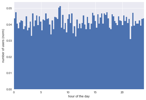
Since the application is world wide spread, we could use a uniform user distribution in the 24h.
hit = np.random.uniform(0,24,size=10000)
plt.hist(hit, normed=True, histtype='stepfilled', bins=100)
_ = plt.xlabel('hour of the day')
_ = plt.ylabel('number of users (norm)')
_ = plt.xlim([0,24])
plt.savefig('uniform.png', bbox_inches='tight')
plt.show()
However, let’s do something more interesting and focus on a single time-zone (just to have a bit of fun). Basing on my experience, there are usually 3 moments for phisical activity:
- early in the morning
- lunch break
- after work
Most of the people play sport after work. Not many do it early in the morning, especially if we are not considering jogging.
hit_gaussian_afternoon = np.random.normal(17.30,2,37500)
hit_gaussian_early = np.random.normal(7.30,1,2500)
hit_gaussian_midday = np.random.normal(11,2,10000)

hit = np.concatenate((hit_gaussian_afternoon,hit_gaussian_early))
hit_gaussian = np.concatenate((hit,hit_gaussian_midday))

plt.hist(hit_gaussian, normed=True, histtype='stepfilled', bins=100)
_ = plt.xlabel('hour of the day')
_ = plt.ylabel('number of users (norm)')
_ = plt.xlim([0,24])
plt.show()
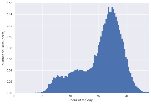
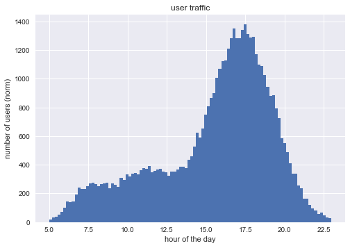
Nice! We can still distinguish a bit the three peaks. Our three joint normal distribution has also some data related to activities before 5 in the morning and after 23. Delete them.
hit_gaussian = hit_gaussian[hit_gaussian>5]
hit_gaussian = hit_gaussian[hit_gaussian<23]

plt.hist(hit_gaussian, normed=True, histtype='stepfilled', bins=100)
_ = plt.xlabel('hour of the day')
_ = plt.ylabel('number of users (norm)')
_ = plt.title('user traffic')
_ = plt.xlim([0,24])
plt.savefig('userGaussian.png', bbox_inches='tight')
plt.show()
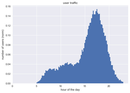
This should be the users traffic (probability density function) during the day. In order to model the Social Feed Loading time we take into account the number of users connected to the system. The loading time will be probably proportional to this number. We will do it in with a sensibility of one hour, but, of course, this would be very sketchy
n = []
for a in hit_gaussian:
    n.append(int(a))

hit_gaussian_round=np.array(n)
bins = np.bincount(np.round(hit_gaussian_round,0))
bins
array([   0,    0,    0,    0,    0,  256,  926, 1414, 1443, 1574, 1933,
       2036, 1931, 2174, 3270, 5178, 6845, 7369, 6101, 4224, 2138,  812,
        266], dtype=int64)
Set the loading time for each user based on two components: - a fixed component proportional to the number of users - a random component following a lognormal distribution
loading_time_fixed = bins/float(10000)

plt.scatter(np.arange(len(loading_time_fixed)), loading_time_fixed)
_ = plt.xlim([0,24])
_ = plt.xlabel('hour of the day')
_ = plt.ylabel('Fixed Loading Time')
_ = plt.title('Fixed Loading time per per hour')
plt.show()
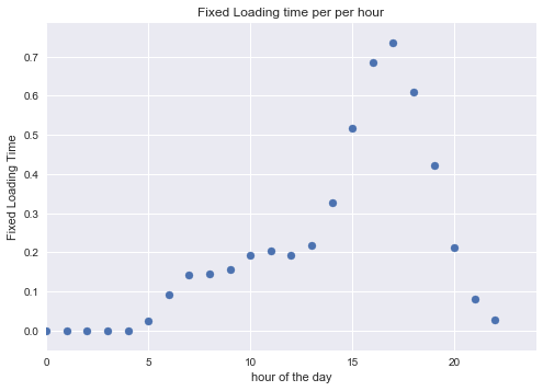
Let’s go back to our users and for each them calculate the loading time. As mentioned it is composed of a fixed amount of time due to congestion and a random amount around 1 second.
These are our users.
plt.hist(hit_gaussian,bins=100)
_ = plt.xlabel('hour of the day')
_ = plt.ylabel('number of users (norm)')
_ = plt.title('user traffic')
plt.show()
Let’s focus on their loading time.
n = []
for a in hit_gaussian:
    n.append(loading_time_fixed[int(a)] + np.random.lognormal(mean=np.log(1),sigma=0.3))

users_waiting_times=np.array(n)
Let’s create a dataframe to handle data more comfortably
df = pd.DataFrame(columns=["TimeTraining","LoadingTime"])
df.TimeTraining = hit_gaussian
df.LoadingTime = users_waiting_times
df.head()
| TimeTraining | LoadingTime | |
|---|---|---|
| 0 | 11.745507 | 1.123004 |
| 1 | 15.675341 | 3.136357 |
| 2 | 14.272109 | 1.646254 |
| 3 | 13.504333 | 0.945362 |
| 4 | 13.719344 | 1.470069 |
df.sample(5000).plot.scatter('TimeTraining','LoadingTime')
_ = plt.title('Loading Time / User Distribution')
plt.show()
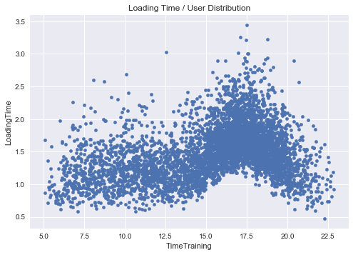
Probably, the variance of the loading time is also proportional to the number of users that are connected and, hence, somehow, to the fixed loading time.
n = []
for a in hit_gaussian:
    n.append(loading_time_fixed[int(a)] + loading_time_fixed[int(a)]* np.random.lognormal(mean=np.log(1),sigma=0.3)*2)
    # I' ve also multiplayed by two to make it a bit smoother

users_waiting_times=np.array(n)
df.TimeTraining = hit_gaussian
df.LoadingTime = users_waiting_times
df.sample(5000).plot.scatter('TimeTraining','LoadingTime')
_ = plt.title('Loading Time / User Distribution')
plt.savefig('LoadingTimeHourRandom.png', bbox_inches='tight')
plt.show()
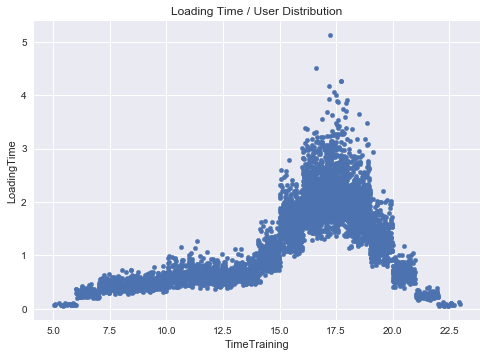
This is better. I do not like those clear steps in the graphs but it is due to our 1-hour discretization binning. Before proceeding to measure the impact of the new features, let’s obtain the loading time per hour with confidence interval, required by the assignment.
df['HourOfTheDay'] = map(lambda x: np.int(x), df['TimeTraining'])
df.head()
| TimeTraining | LoadingTime | HourOfTheDay | |
|---|---|---|---|
| 0 | 11.745507 | 0.642032 | 11 |
| 1 | 15.675341 | 1.281706 | 15 |
| 2 | 14.272109 | 0.847046 | 14 |
| 3 | 13.504333 | 0.572083 | 13 |
| 4 | 13.719344 | 0.820416 | 13 |
ax = sns.boxplot(x="HourOfTheDay", y="LoadingTime", data=df)
plt.savefig('ConfInterval.png', bbox_inches='tight')
plt.show()
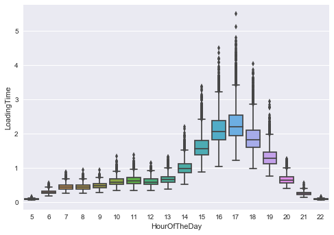
(Question G) We can see higher average LoadingTime but also much more unpredictivity in the rush hours (whether the new feature is adopted or not) ).
Let’s regenerate the data taking into account the users with the feature.
hit_gaussian_feature = np.random.choice(hit_gaussian, size=25000)
hit_gaussian_NoFeature = np.random.choice(hit_gaussian, size=25000)
print(r.mean())
print(feature.mean())
1.39033318677
1.40183209365
n = []
for a in hit_gaussian_NoFeature:
    n.append(loading_time_fixed[int(a)] + loading_time_fixed[int(a)] * np.random.lognormal(mean=np.log(1),sigma=0.3)*2)
    # I' ve also multiplied by two to make it a bit smoother

r = np.array(n)

n = []
for a in hit_gaussian_feature:
    n.append(loading_time_fixed[int(a)] + loading_time_fixed[int(a)] * np.random.lognormal(mean=np.log(1.01),sigma=0.31)*2)
    # I' ve also multiplayed by two to make it a bit smoother

feature = np.array(n)
Let’s repeat the hypothesis testing, with the same hypothesis and condition as before.
from __future__ import division

perm_replicates = draw_perm_reps(feature, r, mean4perm, 10000)

p = np.sum(perm_replicates >= feature.mean()) / len(perm_replicates)
print('p-value = '+str(p))
p-value = 0.0379
We can reject the null hypothesis even this time, hence the loading time is negatively affected by the new feature with a statistical significance of p = 0.0379.
(Question H) We have just assumed that the loading time is affected by the traffic. At the same time, in real world, loading time, and in general, the performance of an application influences the users. E.g. , an increasing loading time would push some users to try competitor softwares. Testing and measuring the impact is not easy. I would introduce an index measuring the activity of the users in the last month. Then I would look for a relationship between this value and the loading time in the last month.
Let us briefly generate some dummy data.
#Average loading time
users_loading = np.random.lognormal(mean=np.log(1),sigma=0.3, size = 25000)

#Activity index - Made it inversely proportional to the average loading time
activity = []
for user in users_loading:
    activity.append(1/float(user + np.random.rand(1)))

activity = np.array(activity)
activity = activity / np.max(activity)
activity.mean()
0.28881507678082624
Let’s measure now the correlation between the average loading time and the activity index. Of course they are strongly inversely correlated because they are generated one from each other in our dummy data but we are not sure for real data.
In our case, people are more likely to use less the app with high loading times.
np.corrcoef(users_loading, activity)[0,1]
-0.64027410048544564
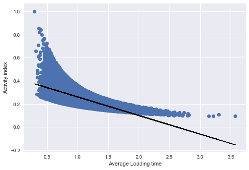
With this hint, we can also somehow predict the activity of the user given his loading time. If, somehow, it increases, the user will probably decrease the activity until quitting.
fit = np.polyfit(users_loading, activity, 1)
fit_fn = np.poly1d(fit)

plt.scatter(users_loading, activity)
plt.plot(users_loading, fit_fn(users_loading), '--k')
_ = plt.xlabel('Average Loading time')
_ = plt.ylabel('Activity index')
plt.savefig('activityWaiting.png', bbox_inches='tight')
plt.show()
Another way to be sure about the results is, again, statistical hypothesis testing. I would compare the average loading time (per user) of the users who quit and the users that are still active.
As before, I would run a permutation test to measure which is the possibility to have a more extreme difference.
inactive_loading = np.random.lognormal(mean=np.log(1.05),sigma=0.3, size = 2000)
active_loading = np.random.lognormal(mean=np.log(1),sigma=0.3, size = 20000)

bins = np.linspace(0, 4, 50)
plt.hist(inactive_loading, bins, alpha=0.5, normed = True, label='inactive')
plt.hist(active_loading, bins, alpha=0.5, normed = True, label='active')
plt.legend(loc='upper right')
plt.show()
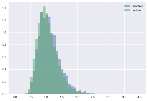
print(inactive_loading.mean())
print(active_loading.mean())
1.10914388061
1.04985877001
from __future__ import division

perm_replicates = draw_perm_reps(inactive_loading, active_loading, mean4perm, 10000)

p = np.sum(perm_replicates >= inactive_loading.mean()) / len(perm_replicates)
print('p-value = '+str(p))
p-value = 0.0
In this way, we strongly reject the null hypothesis which claims that the average loading time do not affect the quitting of a user.
(Question F) Shall we roll back the new feature?
In the end we have seen that it affects the Social feed loading time. We have also mentioned the possible effects of an increasing loading time, which can decrease (in our synthetic data) the activity of users.
On the other end, this feature could be appreciated by the users. The appreciation could mitigate the increased loading time.
Let us imagine the happiness of the users i as H_i. We can think about it as a composition of different factors. The first one, for simplicity, can be seen as the satisfaction related to the features of the application Ho.
Then, as we have hypothesized, there is a Penalty factor related to the loading time of the user P(L_i).
H_i = H_0 - P(L_i)
When does a user quit? When H_i goes below a given threshold alfa. Adding a new feature to the Social Feed:
-
increases the loading time from P(L_i) to P(L_i)’ with ( P(L_i)’> P(L_i))
-
add a factor Hf to the happiness H_i = H_0 + Hf - P(L_i)’ > alfa
Therefore, if H_i > alfa, the user i will keep using the app. The feature appreciation, in fact, could mitigate the increasing loading time effect. Or instead, the increasing loading time delay could be just too small to be noticed.
In the end, not to lose the user i, must hold: Hf > P(L_i)’ - P(L_i)
In a more concrete way, we can measure the activity index already introduced. If, despite the increased loading time, people activity index is increased for the users with the new feature, the feature is appreciated.
Nevertheless, depending on the revenue model, one can think about focusing on few users but more satisfied and willing to spend. If the new feature makes the loading time of the social feed just too slow for some users, they will quit. However, apart from the very sensitive users, most of these people are using old devices. These users, likely, will not spend high amount of money on software applications.
For this reason, letting them quit could be an affordable tradeoff with the aim to increase the conversion-rate (e.g., buy extra services or the premium version of the app) of the most satisfied users.